8 Homework: Week 1
8.1 Instructions
This is homework assignment 1 of 2 for this module. In this assignment, you will apply the concepts learned through Chapter 5 using the MEPS data. There is a total of 36 possible points for this assignment.
You will download a code skeleton for this assignment below by clicking on the red button. This skeleton will provide you an outline for your submission, which will take the form of a R Markdown HTML document.
You will find the homework questions listed in the subsections below. There are a total of 5 parts to this assignment. The questions are intended to be challenging, but doable if you spent the time to learn the material through Chapter 5. Where appropriate, we may provide hints and links to sections in the module that you can reference to help you with the question. All questions are intended to be answerable with the module material provided, but you are encouraged to use any online resources and search engines to come up with solutions to the questions.
8.2 Knitting an HTML Document
To upload your submission as an HTML document, you’ll need to make sure you select Knit to HTML as shown in the graphic below:

8.4 Homework Questions:
8.4.1 Question 1 (2pts):
In Chapter 2, we introduced you to the MEPS data, documentation, and codebook.
Use the codebook to determine what the variable HIDEG refers to, and list all the possible values it could take on along with the unweighted record count for each possible value.
Then, describe using words how you would verify the record count for each value of HIDEG using R if HIDEG were a field in the MEPS data subset that we’ve been using in this module.
8.4.2 Question 2 (2pts):
It is common practice in analytics to try to find external data sources to validate the accuracy of the data you’re working with.
Take, for example, the RACETHX field in the MEPS data.
Use group_by() and summarize() to calculate the sum of the Person-Weight field (PERW18F) when grouping by Race (RACETHX).
Use the codebook to confirm your result.
Explain how you confirmed your result using the codebook.
Then, go online and try to find the population distribution of the 2020 United States Census by Race.
Do the person weights in the MEPS data align with what you found online from the 2020 Census?
8.4.3 Question 3 (5pts):
Create a new dataframe, called hw_df_1 by performing the following manipulations, all in one step, using the pipe %>% to chain commands together:
- Keep only the
DUPERSID,AGE42X, andADBMI42fields - Remove any individuals who have a negative age
- Sort the dataframe such that the highest values of
ADBMI42are at the top - Keep only the first 10 rows of the new dataframe
- Create a new column called
BMI_2that is equal to theADBMI42field rounded to the nearest whole number
Then use the head() function to print the first few results of the new hw_df_1 dataframe.
8.4.4 Question 4 (6pts):
Create a another new dataframe, called hw_df_2 by performing the following manipulations, all in one step, using the pipe %>% to chain commands together:
- Only include individuals with a
POVCAT18status of “LOW INCOME” or “POOR/NEGATIVE” - Simplify your dataframe such that it only includes the fields
POVCAT18,RTHLTH42, andTOTEXP18 - Remove any invalid values for your three remaining fields
- Calculate average medical expenditures by Poverty Category and Perceived Health Status
- Calculate median medical expenditures by Poverty Category and Perceived Health Status (hint: use the
median()function instead of thesum()function) - Calculate the 75th percentile of medical expenditures by Poverty Category and Perceived Health Status (hint: use the
quantile()function instead of thesum()function. Note that you’ll need to somehow tell thequantile()function to use a percentile of 0.75. Remember to use?quantile()to pull up the help menu)
Then use the head() function to print the first few results of the new hw_df_2 dataframe.
8.4.5 Question 5 (10pts):
You are interested in seeing which fields in the MEPS data are associated with receiving a flu shot.
Create a grouped bar chart that shows the percentage of individuals receiving a flu shot by whether or not an individual has a usual source of care (HAVEUS42) and their insurance coverage status (INSCOV18).
HAVEUS42 should be on the x-axis, and INSCOV18 should be split out in the legend.
As part of this exercise, you will also use a custom color palette that we give below you called gopher_colors.
These hex-colors were taken from the following image:

gopher_colors = c("#7A0019", "#FCD131", "#515151")As a hint, refer back to the “Grouped Bar Chart with Percentages” section of Chapter 5 on Data Visualization.
In your grouped bar chart, make sure to do the following:
- Successfully create a grouped bar chart of Flu Shot Percentages by the Usual Source of Care and Insurance Coverage fields
- Remove invalid values
- Use the
gopher_colorscustom color palette as defined above - Include appropriate labels for the x-axis, y-axis, and title
- Your y-axis scale should be in percentages
Once you create your bar chart, explain two observations that you can make from your chart.
8.4.6 Question 6 (11pts):
8.4.6.1 Part 1:
Now you are interested in communicating visually how average medical expenditures vary based on Body Mass Index (BMI). In order to do so, you want to summarize Average Medical Expenditures by your own custom BMI categories. You will use the following classification schedule to define your BMI categories:
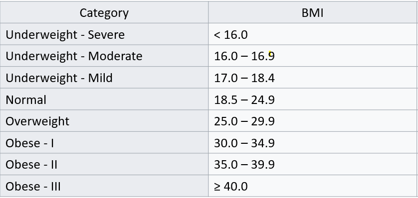
In part 1 of this question, you are to specifically use the cut() function to code these BMI categories.
Then create a bar chart that shows the average medical expenditures by your BMI classification.
For a hint, refer back to the “Bar Chart” section of Chapter 5 on Data Visualization.
In your bar chart, you should:
- Successfully create a bar chart (either vertical or horizontal) that shows average medical spend by BMI category
- Remove any invalid values
- Include labels for your x-axis, y-axis, title, and legend
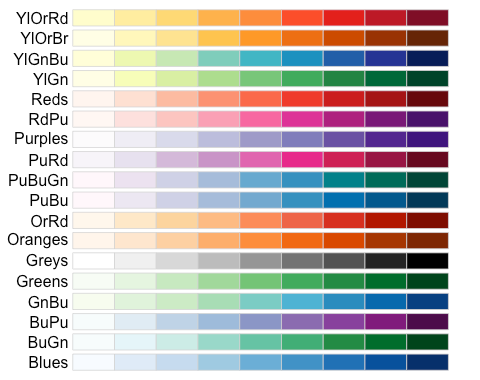
- Use one of the following color scales from the
R Color Brewerpackage (for a hint, you will want to use the `scale_fill_brewer() argument that was used in the “Grouped Bar Chart” section of Chapter 5 on Data Visualization and change the name of the palette.)
8.4.6.2 Part 2:
In part 2 of this question, you are to create a bar chart that plots the same information as in Part 1, except instead of using the cut() function, you will use a case_when() statement to create the new BMI-range field according to the classification schedule above.
Again, your bar chart should plot the exact same information as in Part 1, although you must use the case-when function and you must also use a different color palette.
8.4.6.3 Part 3:
Finally, what do you notice that is different between using cut() as compared to case_when()?
Which function seems to be preferable here? Explain.
8.4.7 Question 7 (5 Bonus Pts):
Question 7 is a bonus question. Any points earned in this section will offset points lost in questions 1-6 above, with a max possible score of 100% for the assignment (i.e. bonus points can’t put you above 100% for the assignment if you get questions 1-6 perfectly correct).
The goal of this question is to test your Google and problem solving skills to create a pie chart using ggplot2 - something we haven’t done yet.
8.4.7.1 Part 1
Create a new dataframe, called pie_data, where you summarize the count of individuals by their flu shot status (ADFLST42).
8.4.7.2 Part 2
Create a pie chart that shows the distribution of individuals who have received, or not received, or have invalid flu shot status.
As a hint, you may want to explore the R Graphy Gallery from earlier to get some ideas.
Your plot should use ggplot2.
If you absolutely cannot get a pie chart to work with ggplot2, you are encouraged to try any other methods you can find online.