4 Manipulating Data
4.1 Motivation
In the first chapter of this module, we talked about the general Data Science Process and the common themes that are found across any data analysis work. In Chapter 2 and Chapter 3, we introduced you to the MEPS dataset and how to import the data into R. In doing so, we covered the first general step of the Data Science Process - collecting or obtaining our data. In this chapter, we begin to address the next steps in the Data Science Process - manipulating our data and exploring our data.
4.2 Primer on Data Manipulation:
There are lots of ways to describe the general idea of manipulating data. You may hear terms like data cleansing, data pre-processing, and data wrangling. While you could argue that each of these terms are technically slightly different, they all get at the general idea that your data needs to be in a usable format before you can perform analyses and modeling on it.
For instance, real world data often does not come in a format that is immediately usable, especially if the data entry is performed by humans (think about someone entering in their own address). Take this example image below, and think of all the things that would make this piece of data difficult to use:
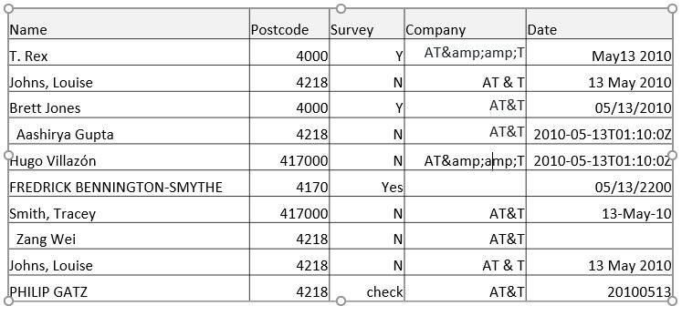
To name a few:
- The names are in multiple cases, have special characters, are in varying orders, and varying number of spaces
- The post codes have varying number of digits
- The survey column has multiple values that both correspond to a value of “Yes” or “Y”
- The date column has dates that are in many different formats
Luckily for us, our MEPS data has already gone through pretty thorough data cleansing and validation processes, and is available to us in a relatively clean format, so we don’t have to worry about a lot of these data pre-processing issues. When you begin your careers, if you work at large corporations there will likely be entire departments of data engineers whose responsibility it is to provide the rest of the organization with as clean of data as possible. Otherwise, if you do have to work with messy data such as the above, you can often spend as much time manipulating the data as all other parts of the data science process combined!
4.3 Dplyr Intro
In this chapter, we will focus on the very basics of data manipulation and transformation using one of the most important packages from the tidyverse: dplyr.
dplyr will also help us begin to explore and summarize our data.
Make sure you have the Tidyverse loaded in your R environment.
4.3.1 What is dplyr
dplyr is one of the core packages of the tidyverse, and is one of the most widely used packages in the R ecosystem.
You can think of dplyr as a package that allows for many of the basic data transformation techniques any Actuary will need in order to take raw data and transform it into usable data for an analysis.
For those familiar with SQL, you will notice many parallels to SQL statements.
Note that SQL knowledge is not necessary for this course, but we may make connections to SQL where appropriate since it is the most widely used language to query and manipulate data.
dplyr itself is almost a ‘sub-language’ of R that requires practice to get the hang of, but once you do, it will make performing complex data transformations simple, succinct, and easy to read.
4.3.2 dplyr foundations
dplyr is predicated on the use of 6 main functions or ‘verbs’:
-
filter(): is used to pick observations/rows in a data frame based on their values (you can think of filter as a “WHERE” clause in SQL) -
arrange(): is used to reorder the rows in a data frame (parallel in SQL would be “ORDER BY”) -
select(): is used to pick variables/columns in a data frame (parallel in SQL would be “SELECT” statement) -
mutate(): is used to create new variables/columns based on other columns in the data frame -
slice(): is used to choose rows based on their location in the data frame -
summarize(): is used to collapse many values down to a single summary value (think of it being used like ‘sum(x) as x’ in a SQL grouped summary statement)
Additionally, there is a seventh function, group_by() that can be used in conjunction with the above functions.
If you pay attention to the bolded text above, you’ll notice that the filter(), arrange() and slice() functions work on rows in your dataset, whereas the select() and mutate() functions work on the columns or fields in your data.
The summarize() function is unique in that it works on groups of rows.
4.3.3 Learning the Basics of the dplyr Package
In this lesson, we’ll walk through the basics of the dplyr package and then you’ll apply and practice using dplyr in your homework assignment.
If you’re interested in a primer, or another document to refer to along the way, I encourage you to check out this Intro to Dplyr post by Joshua Ebner at Sharpsight Labs (estimated read time: 30min-1hour).
This tutorial will walk you through some basic examples of how to use dplyr to transform data using the starwars dataset that comes with the dplyr package.
4.4 Getting Started
To start learning and using the dplyr package, we’ll practice with the MEPS dataset you downloaded and imported into R in Chapter 3.
First, make sure this dataset is loaded:
meps <- readr::read_csv(file = "C:/Users/my_username/Desktop/Data/MEPS.csv",
                                  col_types = cols(
                                  DUPERSID = col_character(),
                                  PANEL = col_character()))
Next, we’ll practice using each of the main dplyr verbs in the context of the MEPS data.
4.5 Using ‘select()’ to pick specific columns
Imagine you had no familiarity with the MEPS dataset, and you wanted to know what columns (often referred to as fields) were in the data.
It’s common in actuarial practice to work with sets of data that have hundreds of fields, and maybe you know you’re only interested in five of them for your analysis.
In this case, it may be useful to select only these handful of columns and store them in a new dataframe to make the data more manageable.
This would be a perfect use case for the select verb, in which you would use this verb to pick only the specific columns that you’re interested in.
Let’s first look at all the possible columns in the MEPS data using the colnames() function.
colnames(meps)
#>  [1] "DUPERSID"   "VARPSU"     "VARSTR"     "PERWT18F"
#>  [5] "PANEL"      "ADFLST42"   "AGE42X"     "AGELAST"
#>  [9] "SEX"        "RACETHX"    "INSCOV18"   "SAQWT18F"
#> [13] "ADGENH42"   "AFRDCA42"   "FAMINC18"   "MNHLTH42"
#> [17] "POVCAT18"   "POVLEV18"   "RTHLTH42"   "HAVEUS42"
#> [21] "REGION42"   "TOTEXP18"   "HIBPDX"     "DIABDX_M18"
#> [25] "ADBMI42"    "ADRNK542"
Let’s say you’re only interested in the columns DUPERSID, PANEL, AGE42X, FAMINC18, REGION42, and TOTEXP18.
To retrieve only these columns and store them in a new dataframe called meps_mini, you would code the following:
meps_mini <- dplyr::select(meps,
                               DUPERSID,
                               PANEL,
                               AGE42X,
                               FAMINC18,
                               REGION42,
                               TOTEXP18)
meps_mini # will print first few rows of the new dataframe, meps_mini
#> # A tibble: 30,461 × 6
#>    DUPERSID   PANEL AGE42X FAMINC18 REGION42 TOTEXP18
#>    <chr>      <chr>  <dbl>    <dbl>    <dbl>    <dbl>
#>  1 2290001101 22        26    32000        2     2368
#>  2 2290001102 22        25    32000        2     2040
#>  3 2290002101 22        33    55000        2      173
#>  4 2290002102 22        39    55000        2        0
#>  5 2290002103 22        11    55000        2      103
#>  6 2290002104 22         8    55000        2        0
#>  7 2290002105 22         4    55000        2        0
#>  8 2290002106 22         2    55000        2       63
#>  9 2290003101 22        36   258083        2      535
#> 10 2290003102 22        36   258083        2     7023
#> # … with 30,451 more rows
4.5.1 A Note on the Pipe Operator: %>%
One of the more useful ways to use dplyr is with the pipe operator.
The pipe operator looks like this: %>% ,and it is common practice to use the pipe operator to “pipe” dplyr commands together.
You may hear it referred to as “chaining” dplyr commands as well.
The pipe operator allows you to combine multiple commands in a row, such that the output of one dplyr function becomes the input of the next.
This allows you to combine many complex data transformation steps into one sequence of commands that makes your code easy to read and follow.
We’ll give a very basic example here using only select() statements, but later in the module we’ll start chaining or piping together several commands using the other dplyr verbs as well.
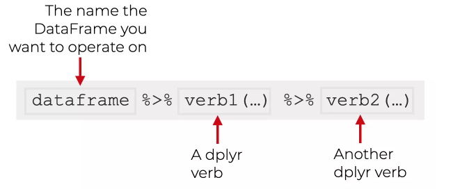
When you are using the pipe operator, you should first think of it as being synonymous with the word “then.”
The graphic below outlines the basic idea.
You start with a dataframe (i.e. the MEPS data), “then” you apply a dplyr verb to transform that data, “then” you apply another dplyr verb to transform the data further.
See how we replaced the pipe operator, %>% with the word “then”?
For example, say you wanted to start with the original MEPS data, “then” you wanted to retrieve the same five columns as above, and “then” you decide you only want the DUPERSID and PANEL fields.
You would code the following:
meps_mini2 <- meps %>%
  dplyr::select(DUPERSID,
                 PANEL,
                 AGE42X,
                 FAMINC18,
                 REGION42,
                 TOTEXP18) %>%
  dplyr::select(DUPERSID, PANEL)
See how this creates a chain of commands that ultimately results in our desired output of a two-column dataframe consisting of the DUPERSID and PANEL fields?
Note that I only needed to specify the name of the original dataframe (meps) a single time in the first line of code, and then that dataframe was fed into the next two lines of code.
Now in this case, the second line of code is redundant and you could have just directly retrieved the DUPERSID and PANEL in a single select() statement.
But, the intention here was to describe how the pipe operator works to chain several commands together.
4.5.2 Practice Exercise 1:
- Create a new data frame, called
meps_ex_1, which only includes theSEX,RACETHX, andADBMI42fields from themepsdataset by using theselect()function along with the pipe operator,%>%.
4.6 Using ‘arrange()’ to reorder the rows of a dataframe
The arrange() verb is used to sort dataframes on one or multiple columns.
Let’s practice sorting the MEPS dataset in conjuction with the select() function and the pipe %>% operator from above.
We’ll create a new dataframe called “meps_sorted” in which we’ll use the select() function to pick a few columns, and then sort the dataframe based on one of the columns.
We then use the head() and tail() functions to look at the first 6 and last 6 rows of the new dataframe.
meps_sorted <- meps %>%
  dplyr::select(DUPERSID, AGE42X, FAMINC18, TOTEXP18) %>%
  dplyr::arrange(TOTEXP18)
head(meps_sorted)#> # A tibble: 6 × 4
#> DUPERSID AGE42X FAMINC18 TOTEXP18
#> <chr> <dbl> <dbl> <dbl>
#> 1 2290002102 39 55000 0
#> 2 2290002104 8 55000 0
#> 3 2290002105 4 55000 0
#> 4 2290006101 51 108168 0
#> 5 2290006102 30 108168 0
#> 6 2290006103 28 11000 0
tail(meps_sorted)#> # A tibble: 6 × 4
#> DUPERSID AGE42X FAMINC18 TOTEXP18
#> <chr> <dbl> <dbl> <dbl>
#> 1 2292785101 65 87400 386185
#> 2 2290605101 69 12948 389089
#> 3 2322825102 38 66177 414532
#> 4 2299680102 48 173805 450168
#> 5 2297686102 53 130000 550741
#> 6 2290197102 44 61000 807611What do you notice when you run head() and tail() on the meps_sorted dataframe?
(Alternatively, you could run View(meps_sorted) and scroll through the data.)
You should notice that the dataset now only contains four fields, and is now sorted in ascending order based on the TOTEXP18 field.
Note that the default of the arrange() function is to sort in ascending order.
If we want to sort in descending order, we’ll use the desc() function within the arrange() function.
It looks like this:
head(meps_descending)#> # A tibble: 6 × 4
#> DUPERSID AGE42X FAMINC18 TOTEXP18
#> <chr> <dbl> <dbl> <dbl>
#> 1 2290197102 44 61000 807611
#> 2 2297686102 53 130000 550741
#> 3 2299680102 48 173805 450168
#> 4 2322825102 38 66177 414532
#> 5 2290605101 69 12948 389089
#> 6 2292785101 65 87400 386185
tail(meps_descending)#> # A tibble: 6 × 4
#> DUPERSID AGE42X FAMINC18 TOTEXP18
#> <chr> <dbl> <dbl> <dbl>
#> 1 2329641105 18 18285 0
#> 2 2329642104 10 0 0
#> 3 2329653103 62 50000 0
#> 4 2329654102 52 181125 0
#> 5 2329655102 79 213564 0
#> 6 2329658102 40 76294 0Now, we see that the data is sorted in descending order based on the TOTEXP18 field.
Finally, we can sort on multiple columns at once.
If we wanted to create a new dataframe called “meps_multi_sort” that is sorted first in descending order by FAMINC18, and then in ascending order by AGE42X, it would look like this:
meps_multi_sort <- meps %>%
  dplyr::select(DUPERSID, AGE42X, FAMINC18, TOTEXP18) %>%
  dplyr::arrange(desc(FAMINC18), AGE42X)
Note that we only performed sorting on numerical columns, but sorting also works for character columns.
In the case of character columns, arrange() will sort in alphabetical order by default, and using desc() with arrange() will sort in reverse alphabetical order.
4.7 Using ’filter()` to subset rows in a data frame
The filter() function allows us to subset or “pick” specific rows out of a data frame based on certain conditions that we define.
For example, let’s say we wanted a new data frame that only had rows in which a person’s age was equal to 25.
In this case, we would be filtering the data based on the condition that a person must be 25 years old.
The code would look like this:
Now, if you look at the tentyfive_only data frame, you should only see values of “25” in the “AGE42X” column.
Note that in order to filter the data frame, we had to use the == operator to test for equality.
Pay attention here that in order to test for equality you need to use two equal signs, not one.
A common error when first learning R is to a single equal sign = instead of two equal signs == when testing for equality.
When this happens R will give you an error.
Under the hood, you can think of this code as R going through the data frame row-by-row, and testing whether the Age value for that row is equal to “25”. For each row that this is true, that row will be returned in the resulting filtered data frame. Each row in which this comparison is false will not be returned in the resulting data frame.
In addition to ==, there are several other comparison operators that you can use to effectively filter data.
-
>or>=- Filters for “greater than” or “greater than or equal to”, respectively -
<or<=- Filters for “less than” or “less than or equal to”, respectively -
!=- Filters for “not-equal-to”
Let’s see how a couple of these could be used in our meps data.
Let’s create a new data frame called fam_income_100k_plus which will only include rows in which a person’s family income is greater than or equal to $100,000.
We’ll use the >= comparison operator to do this.
fam_income_100k_plus <- meps %>%
  dplyr::filter(FAMINC18 >= 100000)

summary(fam_income_100k_plus$FAMINC18)
#>    Min. 1st Qu.  Median    Mean 3rd Qu.    Max.
#>  100000  118924  143870  165244  194545  583219
You’ll now notice that the minimum family income in this new data frame is \(100,000. Note that we used the dollar-sign here, `\)`, to reference a specific field within a data frame.
What about if we wanted a data frame that included all regions except the Northeast.
First, we’d look in the MEPS codebook for the REGION42 variable and find the following:
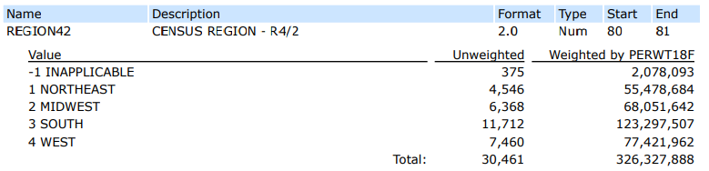
This tells you if you want to remove individuals in the Northeast, you need to remove individuals with a REGION42 value of “1”.
We would then use the != or “not-equal” comparison operator to do this.
We can then use the unique() function to check to make sure the filtering worked correctly (you should not see any values of “1” anymore).
non_northeast <- meps %>%
  dplyr::filter(REGION42 != 1)

unique(non_northeast$REGION42)
#> [1]  2  3  4 -1
4.7.1 Logical Operators with filter()
If you want to combine multiple filtering criteria in a single statement, you’ll need to understand logical or “Boolean” operators in R:
-
&- stands for “and” -
|- stand for “or” -
!- stands for “not”
Boolean operators are common in every coding language. The Venn diagrams below shows the complete set of Boolean operations. “X” is the circle on the left, and “Y” is the circle on the right. The shaded region is the result that is returned from each Boolean operation.
Let’s practice using some of these. For example, let’s say we wanted to filter our MEPS data to include only the rows where the Region is the Northeast AND the age of the individuals is at least 50. To do this, we would write:
The filter() function allows you to separate “AND” conditions with a comma instead of typing &.
For example, the following piece of code would do the exact same as our code above:
# Separate "AND" conditions with commas
northeast_and_50_plus_alternative <- meps %>%
  dplyr::filter(REGION42 == 1,
                AGE42X >= 50)
Now let’s suppose you wanted a data frame that includes either Northeast OR Midwest individuals, and no others.
To create this data frame, you would use the | operator for “OR”.
northeast_or_midwest <- meps %>%
  dplyr::filter(REGION42 == 1 | REGION42 == 2)

unique(northeast_or_midwest$REGION42)
#> [1] 2 1
This code would read as “return a new data frame consisting of the rows in which Region is equal to 1 (Northeast) OR Region is equal to 2 (Midwest).” Note that we had to write REGION42 == twice here for the two conditions.
You can get around having to write multiple conditions out by using the %in% operator (pronounced the “IN” operator).
For example, the following code would do the exact same as the above.
northeast_or_midwest_alternative <- meps %>%
  dplyr::filter(REGION42 %in% c(1, 2))

unique(northeast_or_midwest_alternative$REGION42)
#> [1] 2 1
This second approach is recommended for instances in which you may have several items (in this case Regions) that you want to include in your filter statement. Note that in order to use the %in% operator, we had to create a vector in R using the c() function.
4.7.2 Putting it all together
Now that we’ve seen several examples of how to filter data frames in R, let’s try a challenge problem that incorporates many of these concepts at once.
Let’s say you are asked to return a data frame that has the following requirements:
- Includes only records in which the person is FEMALE, and
- Includes only records in which the person is at least 35 years old but less than 38 years old, and
- Includes only records in which the person has a perceived mental health status of “Excellent” or “Very Good”, and
- Does not include any records in which the Region is in inapplicable or in the South or West regions.
First, let’s look at the MEPS codebook to make sure we know which values to use from each column.
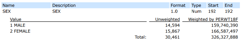
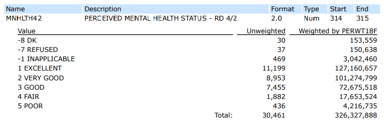
From this, we know that in order to select females, we’ll need to filter on a SEX value of 2.
Additionally, to filter on individuals with an Excellent or Very Good perceived mental health status, we’ll need to filter MNHLTH42 to include the values of 1 OR 2.
Pay attention to where the ands and ors are in the above requirements. Here is how you might write the code to return a data frame with those four requirements:
challenge_example <- meps %>%
  dplyr::filter(SEX == 2,
                AGE42X >= 35,
                AGE42X < 38,
                MNHLTH42 %in% c(1,2),
                ! REGION42 %in% c(-1, 3,4))

unique(challenge_example$SEX)
#> [1] 2
unique(challenge_example$AGE42X)
#> [1] 35 37 36
unique(challenge_example$MNHLTH42)
#> [1] 1 2
unique(challenge_example$REGION42)
#> [1] 2 1
Use View(challenge_example) to scan the resulting dataset to confirm that you think the logic worked.
4.8 slice() - choose rows based on location
slice() allows you to pick out or select specific rows by their row-number in a dataset.
We’ll demonstrate two very simple use cases of the slice() verb.
4.8.1 Using slice() to select rows based on their integer location
For our first example, lets suppose you were interested in creating a new data frame that only included rows 5 through 10 of the meps dataset. In order to specifically select only these rows, you would write the following:
If you happen to know how to subset in base R using row indices, you could perform the equivalent task without using the dplyr package:
rows_5_thru_10_alternative <- meps[5:10,]
4.8.2 Using slice() to select minimum or maximum values
Another common use of the slice() verb is to select minimum or maximum values out of a data frame using slice_min() or slice_max().
Let’s say you wanted to find the 10 rows with the highest dollar amount for total medical expenditures in 2018.
In our meps data, the TOTEXP18 field has the individual’s total expenditures for the year of 2018.
In order to select the 10 rows with the highest medical expenditures, you could write the following:
Alternatively, if you remember from the arrange() section above, you could write it this way:
As you can see, there’s often multiple ways to code the same thing.
The slice() verb can also be used to select samples out of a data frame.
Type ?dplyr::slice in the Console to learn more about slice(), if interested.
4.9 Using mutate() to modify or add new columns
If you need to modify existing columns in your data, or if you need to create new columns that are functions of other fields in your data, you would use mutate().
4.9.1 Modifying currently existing fields
In this example, we’ll make a modification to a currently existing field by using the mutate() function along with round().
Let’s say we wanted to simplify the family income values to be rounded to the nearest one-thousand.
Additionally, we want these new, rounded values, to override what was previously in the family income field.
To do this, we need to mutate the FAMINC18 field by rounding it to the nearest one-thousand.
Note that inside the round() function, we use “-3” to specify rounding to the nearest one-thousand.
If you wanted to round a value to the nearest whole number, you would use a “0” instead of the “-3”, and if you wanted to round a value to the one-hundreths place, you would use the value “2”, and so forth.
See ?round() if you would like more information on this function.
4.9.2 Adding a new column
You can also use mutate() to add a new column to your data frame.
Often times, this new column will be a function of an existing column.
For example, let’s say you know that inflation has increased 20% from the year 2000 to 2018, and so you want to try to convert the 2018 medical expenditure dollars to their year-2000 equivalent by adjusting for inflation.
Use View(modified_data2) to check the new year-2000 medical expenditure column, called “year_2000_med_exp”.
4.9.3 Challenge Example - Using case_when() with mutate()
In this example, we’ll practice use case_when() statements in conjunction with mutate() to create new columns based on conditions and values of other columns.
A case_when() statement allows to create a new column or modify an existing column using multiple if-then criteria.
It is best illustrated with an example.
Let’s say you’re working with the MEPS data, and you’re tired of going back and forth in the codebook to look up what the values of different fields mean.
One solution would be to use a case_when() statement to manually override the values of a given field.
For example, let’s re-code the REGION42 field so that it’s values correspond to the actual regions instead of integers.
First, you might check what the possible values of the REGION42 field are to make sure you’re not missing any:
Next, we re-write the 5 possible values based on their definition in the codebook:
meps_region_override <- meps %>%
  dplyr::mutate(
    REGION42 = case_when(
      REGION42 == 1 ~ "NORTHEAST",
      REGION42 == 2 ~ "MIDWEST",
      REGION42 == 3 ~ "SOUTH",
      REGION42 == 4 ~ "WEST",
      REGION42 == -1 ~ "INAPPLICABLE"
    )
  )

unique(meps_region_override$REGION42)
#> [1] "MIDWEST"      "SOUTH"        "NORTHEAST"
#> [4] "WEST"         "INAPPLICABLE"
table(meps_region_override$REGION42) # to show counts of each value
#>
#> INAPPLICABLE      MIDWEST    NORTHEAST        SOUTH
#>          375         6368         4546        11712
#>         WEST
#>         7460
In this example, we used mutate() along with case_when() to override the REGION42 field by doing the following:
-
If
REGION42is equal to 1, then assign it to the value of “NORTHEAST”, -
Else, if
REGION42is equal to 2, then assign it to the value of “MIDWEST”, -
Else, if
REGION42is equal to 3, then assign it to the value of “SOUTH”, -
Else, if
REGION42is equal to 4, then assign it to the value of “WEST”, -
Else, if
REGION42is equal to -1, then assign it to the value of “INAPPLICABLE”
Now, anytime you wish to use the REGION42 field, you can directly use the actual region names instead of the numerical values.
If you are interested in learning more about mutate(), please see Section 5.5 of R for Data Science.
4.10 Using group_by() and summarize() to create grouped summaries
The combination of group_by() and summarize() will be one of the most important and frequently used combinations that you will use as an actuary.
These functions allow you to calculate grouped summaries of data, which is extremely useful when summarizing data.
Let’s consider a very basic example of a grouped summary to introduce the concept. If someone asked you to take the MEPS data and calculate the total medical expenditures by region, how would go about this conceptually? You would first split the data between each of the regions, and then within each region, you would sum up the total medical expenditures. This is the concept of a grouped summary - you would be grouping-by region and summarizing the medical spend
Let’s convert this idea to code using our new dataframe from the prior section where we overrode the REGION42 field:
region_summary <- meps_region_override %>%
  dplyr::group_by(REGION42) %>%
  dplyr::summarize(Total_Med_Exp = sum(TOTEXP18))

region_summary
#> # A tibble: 5 × 2
#>   REGION42     Total_Med_Exp
#>   <chr>                <dbl>
#> 1 INAPPLICABLE       1207928
#> 2 MIDWEST           44220265
#> 3 NORTHEAST         32506175
#> 4 SOUTH             67390073
#> 5 WEST              40301822
What you are left with is a new data frame that consists of the total medical spend summarized by region.
The power and usefulness of grouped summaries is again most easily shown through another example case.
Imagine you are an actuarial analyst and your boss is interested in trying to understand what factors lead to higher average medical expenditures. You hypothesize that medical expenditures may be related to high blood pressure and diabetes, as well as a person’s perceived mental health status. Your boss then requests you to pull average medical expenditures to see if your hypothesis appears to be true. How would you go about fulfilling your boss’s request?
If you were to break down this request into steps, it might look like this:
- Re-code the variables for high blood pressure status (HIBPDX), diabetes status (DIABDX_M18), and perceived mental health status (MNHLTH42) to values that are easier to read
- Filter the data to exclude inappropriate values for any of these variables
- Calculate total medical expenditures by each of these variables
- Calculate the total number of individuals that fall into each of these combination of variables
- Calculate the average medical expenditure for a person with a given combination of these three variables
- Sort by average medical expenditures, in descending order
Now that we’ve mapped out the steps we need to take, let’s implement the code. We’re going to do all of it in one step, but you can break it up into each of the separate steps if you’d like:
boss_request_1 <- meps %>%

  # Step 1 - Recode Values
  dplyr::mutate(
    HIBPDX = case_when(
      HIBPDX == 1 ~ "YES",
      HIBPDX == 2 ~ "NO",
      HIBPDX %in% c(-15, -8, -7, -1) ~ "REMOVE"
    ),
    DIABDX_M18 = case_when(
      DIABDX_M18 == 1 ~ "YES",
      DIABDX_M18 == 2 ~ "NO",
      DIABDX_M18 %in% c(-15, -8, -7, -1) ~ "REMOVE"
    ),
    MNHLTH42 = case_when(
      MNHLTH42 == 1 ~ "EXCELLENT",
      MNHLTH42 == 2 ~ "VERY GOOD",
      MNHLTH42 == 3 ~ "GOOD",
      MNHLTH42 == 4 ~ "FAIR",
      MNHLTH42 == 5 ~ "POOR",
      MNHLTH42 %in% c(-8, -7, -1) ~ "REMOVE"
    )
  ) %>%

  # Step 2: Filter out undesirable values
  dplyr::filter(
    HIBPDX != "REMOVE",
    DIABDX_M18 != "REMOVE",
    MNHLTH42 != "REMOVE"
  ) %>%

  # Step 3&4: Group by and calculate Total Medical Expenditures
  #   and person-counts for each combination of variables
  dplyr::group_by(
    HIBPDX,
    DIABDX_M18,
    MNHLTH42) %>%
  dplyr::summarize(
    Total_Med_Exp = sum(TOTEXP18),
    person_count = n()
  ) %>%
  ungroup() %>%

  # Step 5: Calculate average medical spend by group
  dplyr::mutate(Average_Med_Exp = Total_Med_Exp / person_count) %>%

  # Step 6: Arrange average spend in descending order
  dplyr::arrange(desc(Average_Med_Exp))
boss_request_1#> # A tibble: 20 × 6
#> HIBPDX DIABDX_M18 MNHLTH42 Total_Med_Exp person_count
#> <chr> <chr> <chr> <dbl> <int>
#> 1 YES YES POOR 2607428 80
#> 2 YES YES FAIR 8198662 330
#> 3 NO YES POOR 384890 18
#> 4 YES NO POOR 2435001 134
#> 5 YES YES VERY GOOD 9053507 509
#> 6 YES YES GOOD 12745207 745
#> 7 NO NO POOR 2711972 173
#> 8 YES NO FAIR 8225327 578
#> 9 YES YES EXCELLENT 6592981 476
#> 10 NO YES GOOD 2865433 233
#> 11 NO YES VERY GOOD 2305117 189
#> 12 NO YES FAIR 801046 67
#> 13 YES NO GOOD 18669536 1757
#> 14 NO NO FAIR 6371278 722
#> 15 NO YES EXCELLENT 1421991 164
#> 16 YES NO VERY GOOD 13615162 1730
#> 17 YES NO EXCELLENT 10516715 1465
#> 18 NO NO GOOD 17732440 3381
#> 19 NO NO VERY GOOD 18165928 4583
#> 20 NO NO EXCELLENT 18176112 5153
#> # … with 1 more variable: Average_Med_Exp <dbl>We did several things here:
- First we used
mutate()andcase_when()to recode the values for High Blood Pressure, Diabetes, and Mental Health Status to more reader-friendly values - Next, we used
filter()to remove any of the rows which contained inapplicable values - Then, we used
group_by()andsummarize()to calculate the total medical spend by High Blood Pressure, Diabetes, and Mental Health Status (Total_Med_Exp = sum(TOTEXP18)) - At the same time, we also used
group_by()andsummarize()to calculate the number of persons falling into each combination of those 3 fields (person_count = n()) - Then, we used
ungroup()to basically tell R that we’ve completed our group-by-and-summarize procedure. This is recommended to put after eachgroup_by()andsummarize()combination if you have other statements that come after the group-by-and-summarize - Next, we created a new column using
mutate(), calledAverage_Med_Exp, by diving theTotal_Mex_Expby theperson_count - Finally, we re-arranged the resulting dataframe such that it was sorted in descending order by the
Average_Med_Exp
What do you notice when you look at the new boss_request_1 dataframe?
Do you think these results help support your hypothesis that higher medical expenditures are associated with high blood pressure, diabetes, and poor mental health?
4.11 Conclusion
If there is one section of the case study to try to best understand, it would be the concepts in this chapter. Data manipulation is a foundational skill that you must become highly proficient in to be a successful actuary or analyst in any data-heavy role. Once you get into your careers, you’ll find that often far more time is spent working to manipulate and clean your data than is spent producing a model. We’ve only scratched the surface here, but have laid the foundation for a basic understanding of what it means to take a set of data and manipulate that data to produce whatever it is you’re interested in.