3 Importing Data
3.1 What is Data Importing
For the first R activity of this module, we will practice reading in, or importing, data from a file. After all, if we can’t get the data into R, we won’t be able to perform any analyses on it. The process of importing data into R may seem like a trivial task if the data is already relatively clean. But, you will likely encounter situations as an Actuary or Data Scientist where you will have to find ways to import messy data into your R environment before you can analyze it. This chapter will go over the basics of importing a relatively clean file.
3.1.1 Prereqs:
In this chapter we’re going to focus on how to use the readr package to read or import files into R.
readr is a core member of a suite of packages called the tidyverse.
The tidyverse collection includes packages that you’re most likely to use in every data analyses, and we will use several other packages from the tidyverse as we work our way through the module.
When you begin your actuarial careers, you may encounter data in many different forms, including Excel files (.xlsx) and Comma-Separated-Value files (.csv). You may also encounter plain text files (.txt), and these files may use specific delimiters to define the boundaries between entries in the data. Or, you may need to connect your R environment to a Database and write queries to pull select data down from the database. Suffice to say, there are many different ways data can be organized that require different methods to capture this data and load it into your R environment.
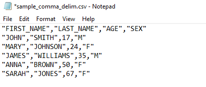
In this chapter, we will focus on one of the most common file layouts, which is the Comma-Separate-Value (CSV) layout. A CSV file is a type of delimited text file that separates the values in the data by using commas. The raw data will typically look something like the example image below, where the first row of the file specifies the column names, and each of the data entries are separated by commas.
If we were to read this example CSV file into R, it would look like this in our environment:
| FIRST_NAME | LAST_NAME | AGE | SEX |
|---|---|---|---|
| JOHN | SMITH | 17 | M |
| MARY | JOHNSON | 24 | F |
| JAMES | WILLIAMS | 35 | M |
| ANNA | BROWN | 50 | F |
| SARAH | JONES | 67 | F |
3.2 Learning the Code
Now that we know the basics of what data importing is, and we’ve seen an example of one of the most common types of file formats, the CSV format, we will practice reading in our own CSV file. The file that we will import is a subset of the 2018 MEPS Household Component - in reality there are over 1,500 columns in the real MEPS consolidated file which can be found here. We will use this example dataset for the rest of the module.
Please download the example MEPS data below, and save the file onto your local computer. Once you have done this, please read Sections 11.1 and 11.2 of R for Data Science to learn the basics of how to import a CSV file into R. Please note the exercises at the end of these two sections are not required.
We will be utilizing the read_csv() function from the readr package.
Note that when you are calling functions in R, you have the choice of calling the function in two ways:
- Using the “full-name” of the function, which uses the syntax
some_package::some_function(), which in our case is,readr::read_csv() - Or, you may just use the name of the function, for example
read_csv(). If you use this approach, you must have already loaded the package that houses the function you intend to use. In this case, you must have loaded the readr package using eitherlibrary(readr)orlibrary(tidyverse). This option allows for shorter syntax, but there are cases where two functions from two different packages could have the same name in which case you would need to use the “full-name” to specify exactly which package has the function you want to use. Using the full-name is always the safest approach to ensure you’re using your intended function.
3.3 Implementing the Code
After reading sections 11.1 and 11.2 of R for Data Science, you should now have a basic understanding of how to import a CSV file into R. In order to now import our MEPS file that you downloaded, we need to define the file path or location on your computer from which R can access the file and load it into your environment. We’ll walk through a couple ways to do this, highlighting differences you’ll need to be aware of between Mac and Windows operating systems.
3.3.1 Windows Users:
First, you need to locate where on your computer you saved the downloaded MEPS file. For a Windows user, maybe you saved the file in a folder called “Data” on your desktop. The Windows file path would then look something like:
- “C:\Users\insert_your_user_name\Desktop\Data”
The following code shows two simple ways to then import the MEPS dataset into your R environment and assign the data to an R dataframe object named “meps”.
Note that if you do not use the file.path() function approach, on a Windows computer you must change the back slashes to front slashes in the file path
3.3.1.1 Option 1:
Feed the absolute path of the MEPS file into the readr::read_csv() function.
Note that R is always case sensitive.
# Note the file path must be surrounded in quotations and you must change back slashes to front slashes

meps <- readr::read_csv("C:/Users/my_username/Desktop/Data/MEPS.csv")
3.3.1.2 Option 2:
Use the file.path() function to define the location of the file:
3.3.2 Mac Users:
The process is similar for Mac users, but the way file paths are defined is a little different. Let’s assume again that you saved your MEPS file onto your Desktop in a folder named “Data”. We’ll walk through two different approaches you can use for Mac. Note that for a Mac, you shouldn’t have to change any back slashes to front slashes in the file path - they should already be front slashes in Mac OS.
3.3.2.1 Option 1:
Feed the absolute path into the readr function.
To find the path of a file on a Mac:
- Navigate to the location of the file in your Finder application
- Right click on the file and then hold down the Option key
- You should see a option that says “Copy ‘MEPS.csv’ as Pathname
- Select this option and then paste that into Rstudio. It should look something like this:
meps <- readr::read_csv("/Users/my_username/Desktop/Data/MEPS.csv")- Option 2: You can use the following shorthand notation if you have the MEPS file saved in a folder called “Data” on your desktop:
meps <- readr::read_csv("~/Desktop/Data/MEPS.csv")If you get stuck, you can Google search “Relative Paths and the Working Directory in R” for articles or videos on YouTube that should help you get going.
3.4 Refining the Code
Now that we’ve successfully loaded the MEPS data into our R environment, we need to check a couple things about our data.
If you look in the upper right window of RStudio, you should see a new dataframe called “meps” in the Environment pane.
Take a minute to explore the data you just imported by either clicking on “meps”, or typing View(meps) in the Console at the bottom. This will open a new window within RStudio to explore your data.
If you want a completely new window to pop up with your data, try running utils::View(meps) instead.
After you have spent a few minutes looking at the data, let’s take a closer look at what types of data are represented by each of the columns.
Type str(meps) in the console.
str(meps)#> spec_tbl_df [30,461 × 26] (S3: spec_tbl_df/tbl_df/tbl/data.frame)
#> $ DUPERSID : num [1:30461] 2.29e+09 2.29e+09 2.29e+09 2.29e+09 2.29e+09 ...
#> $ VARPSU : num [1:30461] 1 1 2 2 2 2 2 2 2 2 ...
#> $ VARSTR : num [1:30461] 2035 2035 2048 2048 2048 ...
#> $ PERWT18F : num [1:30461] 19668 18189 3567 3880 2707 ...
#> $ PANEL : num [1:30461] 22 22 22 22 22 22 22 22 22 22 ...
#> $ ADFLST42 : num [1:30461] 2 1 2 2 -1 -1 -1 -1 2 -1 ...
#> $ AGE42X : num [1:30461] 26 25 33 39 11 8 4 2 36 36 ...
#> $ AGELAST : num [1:30461] 27 25 34 39 11 8 4 2 36 36 ...
#> $ SEX : num [1:30461] 2 1 2 1 1 1 1 1 2 1 ...
#> $ RACETHX : num [1:30461] 2 2 1 1 1 1 1 1 2 2 ...
#> $ INSCOV18 : num [1:30461] 1 1 1 1 1 1 1 1 1 1 ...
#> $ SAQWT18F : num [1:30461] 20810 18207 4351 4134 0 ...
#> $ ADGENH42 : num [1:30461] 2 1 3 3 -1 -1 -1 -1 2 -1 ...
#> $ AFRDCA42 : num [1:30461] 2 2 2 2 2 2 2 2 2 2 ...
#> $ FAMINC18 : num [1:30461] 32000 32000 55000 55000 55000 ...
#> $ MNHLTH42 : num [1:30461] 3 2 3 3 3 3 3 3 3 3 ...
#> $ POVCAT18 : num [1:30461] 3 3 3 3 3 3 3 3 5 5 ...
#> $ POVLEV18 : num [1:30461] 190 190 164 164 164 ...
#> $ RTHLTH42 : num [1:30461] 2 2 3 3 3 3 3 3 2 3 ...
#> $ HAVEUS42 : num [1:30461] 1 1 1 2 1 1 1 1 1 1 ...
#> $ REGION42 : num [1:30461] 2 2 2 2 2 2 2 2 2 2 ...
#> $ TOTEXP18 : num [1:30461] 2368 2040 173 0 103 ...
#> $ HIBPDX : num [1:30461] 2 2 2 2 -1 -1 -1 -1 2 2 ...
#> $ DIABDX_M18: num [1:30461] 2 2 2 2 2 2 2 2 2 2 ...
#> $ ADBMI42 : num [1:30461] 21.4 30.6 28.2 28.7 -1 -1 -1 -1 21.5 -1 ...
#> $ ADRNK542 : num [1:30461] -1 1 -1 2 -1 -1 -1 -1 -1 -1 ...
#> - attr(*, "spec")=
#> .. cols(
#> .. DUPERSID = col_double(),
#> .. VARPSU = col_double(),
#> .. VARSTR = col_double(),
#> .. PERWT18F = col_double(),
#> .. PANEL = col_double(),
#> .. ADFLST42 = col_double(),
#> .. AGE42X = col_double(),
#> .. AGELAST = col_double(),
#> .. SEX = col_double(),
#> .. RACETHX = col_double(),
#> .. INSCOV18 = col_double(),
#> .. SAQWT18F = col_double(),
#> .. ADGENH42 = col_double(),
#> .. AFRDCA42 = col_double(),
#> .. FAMINC18 = col_double(),
#> .. MNHLTH42 = col_double(),
#> .. POVCAT18 = col_double(),
#> .. POVLEV18 = col_double(),
#> .. RTHLTH42 = col_double(),
#> .. HAVEUS42 = col_double(),
#> .. REGION42 = col_double(),
#> .. TOTEXP18 = col_double(),
#> .. HIBPDX = col_double(),
#> .. DIABDX_M18 = col_double(),
#> .. ADBMI42 = col_double(),
#> .. ADRNK542 = col_double()
#> .. )
#> - attr(*, "problems")=<externalptr>You will note that all of the fields have been read into R as “numeric” columns. As a general rule of thumb, you want columns that will be treated like numbers to be read in as numeric columns, and columns that you will treat as descriptors or strings of text to be read in as character columns. In our case, we will be treating a lot of these variables as character strings instead of numbers, so we will need to modify them in some way such that they are treated as characters instead of numbers. We will get to this in more detail in Chapter 4 on Transforming Data.
For now, you will note that the first column, DUPERSID has been read in as a numeric column because the ID column is a series of digits.
In this case, the read_csv() function guessed that you wanted this field to be treated as numeric because it contains only digits.
However, we use ID’s to describe individuals - we don’t use ID’s in the same way that we use numbers.
In other words, you would never add IDs or subtract or multiply, etc. and so this column should be treated as a character column.
The same logic applies to the Panel column.
The Panel simply describes which Panel a person is from - you wouldn’t treat them like numbers and add Panel numbers together.
Therefore, we need a way to tell read_csv() to treat those two columns as character columns instead of numeric columns.
We do this using the col_types() argument within the read_csv() function.
It works like this:
meps <- readr::read_csv(file = "C:/Users/my_username/Desktop/Data/MEPS.csv",
                       col_types = cols(
                         DUPERSID = col_character(),
                         PANEL = col_character()))
Now, if we use the str() function to check the column types of our newly imported dataset, meps, we should see that the DUPERSID, and PANEL columns are now character columns.
And just like that, you now have successfully loaded a CSV file into your R environment and are ready for the next chapter in the module!
str(meps)#> spec_tbl_df [30,461 × 26] (S3: spec_tbl_df/tbl_df/tbl/data.frame)
#> $ DUPERSID : chr [1:30461] "2290001101" "2290001102" "2290002101" "2290002102" ...
#> $ VARPSU : num [1:30461] 1 1 2 2 2 2 2 2 2 2 ...
#> $ VARSTR : num [1:30461] 2035 2035 2048 2048 2048 ...
#> $ PERWT18F : num [1:30461] 19668 18189 3567 3880 2707 ...
#> $ PANEL : chr [1:30461] "22" "22" "22" "22" ...
#> $ ADFLST42 : num [1:30461] 2 1 2 2 -1 -1 -1 -1 2 -1 ...
#> $ AGE42X : num [1:30461] 26 25 33 39 11 8 4 2 36 36 ...
#> $ AGELAST : num [1:30461] 27 25 34 39 11 8 4 2 36 36 ...
#> $ SEX : num [1:30461] 2 1 2 1 1 1 1 1 2 1 ...
#> $ RACETHX : num [1:30461] 2 2 1 1 1 1 1 1 2 2 ...
#> $ INSCOV18 : num [1:30461] 1 1 1 1 1 1 1 1 1 1 ...
#> $ SAQWT18F : num [1:30461] 20810 18207 4351 4134 0 ...
#> $ ADGENH42 : num [1:30461] 2 1 3 3 -1 -1 -1 -1 2 -1 ...
#> $ AFRDCA42 : num [1:30461] 2 2 2 2 2 2 2 2 2 2 ...
#> $ FAMINC18 : num [1:30461] 32000 32000 55000 55000 55000 ...
#> $ MNHLTH42 : num [1:30461] 3 2 3 3 3 3 3 3 3 3 ...
#> $ POVCAT18 : num [1:30461] 3 3 3 3 3 3 3 3 5 5 ...
#> $ POVLEV18 : num [1:30461] 190 190 164 164 164 ...
#> $ RTHLTH42 : num [1:30461] 2 2 3 3 3 3 3 3 2 3 ...
#> $ HAVEUS42 : num [1:30461] 1 1 1 2 1 1 1 1 1 1 ...
#> $ REGION42 : num [1:30461] 2 2 2 2 2 2 2 2 2 2 ...
#> $ TOTEXP18 : num [1:30461] 2368 2040 173 0 103 ...
#> $ HIBPDX : num [1:30461] 2 2 2 2 -1 -1 -1 -1 2 2 ...
#> $ DIABDX_M18: num [1:30461] 2 2 2 2 2 2 2 2 2 2 ...
#> $ ADBMI42 : num [1:30461] 21.4 30.6 28.2 28.7 -1 -1 -1 -1 21.5 -1 ...
#> $ ADRNK542 : num [1:30461] -1 1 -1 2 -1 -1 -1 -1 -1 -1 ...
#> - attr(*, "spec")=
#> .. cols(
#> .. DUPERSID = col_character(),
#> .. VARPSU = col_double(),
#> .. VARSTR = col_double(),
#> .. PERWT18F = col_double(),
#> .. PANEL = col_character(),
#> .. ADFLST42 = col_double(),
#> .. AGE42X = col_double(),
#> .. AGELAST = col_double(),
#> .. SEX = col_double(),
#> .. RACETHX = col_double(),
#> .. INSCOV18 = col_double(),
#> .. SAQWT18F = col_double(),
#> .. ADGENH42 = col_double(),
#> .. AFRDCA42 = col_double(),
#> .. FAMINC18 = col_double(),
#> .. MNHLTH42 = col_double(),
#> .. POVCAT18 = col_double(),
#> .. POVLEV18 = col_double(),
#> .. RTHLTH42 = col_double(),
#> .. HAVEUS42 = col_double(),
#> .. REGION42 = col_double(),
#> .. TOTEXP18 = col_double(),
#> .. HIBPDX = col_double(),
#> .. DIABDX_M18 = col_double(),
#> .. ADBMI42 = col_double(),
#> .. ADRNK542 = col_double()
#> .. )
#> - attr(*, "problems")=<externalptr>3.5 A Quick Note on Using Google and Search Engines
Whether you’re first learning R or you are a daily user with years of experience, the internet is your best friend. One of the biggest benefits of the R language is that there is a huge and active userbase online of people who have written tutorials, answered questions, and faced many of the same problems and questions you will face. In fact, it is almost guaranteed that at some point, someone else has had the exact same problem as you, asked their question online, and it was answered with multiple different ways to solve it. As such, learning how to solve your problems with Google or your preferred search engine is a skill that will help you enormously in R or any other programming language. Here are a few tips for how to best solve your problems online:
- Always include “R” in the search phrase
- If you know what package or function you need to use, include that in the search phrase
- If you know that you need to use the tidyverse to solve your problem, use tidyverse in the search phrase
- Stackoverflow is typically the best website to solve your issues, particularly if your question is very specific or difficult. Stackoverflow is a question-and-answer website for programmers of all types, and your question has more likely than not to have been asked and answered on Stack Overflow at some point. If you see your search engine return a result with a link to Stack Overflow, it’s usually most efficient to start there.
For example, let’s say you hadn’t completed this module, and you wanted to know how to read the DUPERSID column in as a character column instead of a numeric column.
A search phrase you may type into Google would look like: “how to change column type when reading csv file in R with readr tidyverse”.
Note that this search phrase includes what you’re trying to answer, the packages that may help you answer it, and the keyword “R”.
This link was the first search result that came up, and note that it is also from the Stack Overflow website.
After spending a couple minutes reading the user’s questions and the top one or two “upvoted” answers, you would be able to figure out how to change the column type when importing a CSV file in R.