Chapter 8 Statistical inference

In a previous chapter, we learned about estimation: the use of data and statistics to construct the best possible guess at the value of some parameter.

In this chapter, we will pursue a different goal. Instead of estimating the single “most likely” value of the parameter, we will construct statistics that can be used to classify particular parameter values as plausible (could be the true value) or implausible (unlikely to be the true value).

A hypothesis test determines whether a particular value can be ruled out.
A confidence interval determines a range of values that cannot be ruled out.

The set of procedures for constructing confidence intervals and hypothesis tests is called statistical inference.

Chapter goals

In this chapter we will learn how to:

Construct and perform a simple hypothesis test
Construct a confidence interval
Correctly interpret both hypothesis tests and confidence intervals

8.1 Principles of inference

8.1.1 Evidence

The purpose of statistical inference is to systematically account for the uncertainty associated with limited evidence. That is, there are important aspects of the data generating process we do not know. The data provide some evidence about those unknown aspects, but the evidence they provide may not be strong. Statistical inference asks us what statements about the data generating process can be made with confidence based on the data.

Example 8.1 Fair and unfair roulette games

Suppose you work as a casino regulator for the BCLC (British Columbia Lottery Corporation, the crown corporation that regulates all commercial gambling in B.C.). You have been given data with recent roulette results from a particular casino and are tasked with determining whether the casino is running a fair game.

Before getting caught up in math, let’s think about how we might assess evidence:

We might have results from many games, or only a few games.
Our results may have a win rate close to the expected rate for a fair game, or far from that rate.

We can put those possibilities into a table:

Win rate	Many games	Few games
Close to fair game rate	Probably fair	Could be fair or unfair
Far from fair game rate	Probably unfair	Could be fair or unfair

That is, we can make a fairly confident conclusion if we have a lot of evidence, and our conclusion depends on what the evidence shows. But if we do not have a lot of evidence, we cannot make a confident conclusion either way.

In this chapter we will formalize these basic ideas about evidence.

8.1.2 A basic framework

For the remainder of this chapter, suppose we have a data set $D_n = (x_1,x_2,\ldots,x_n)$ of size $n$. The data comes from an unknown data generating process that includes an unknown parameter of interest $\theta$.

Example 8.2 DGP and parameter of interest for roulette

Let $D_n = (x_1,\ldots,x_n)$ be a data set of results from $n = 100$ games of roulette at a local casino. More specifically, let \[x_i = I(\textrm{Red wins})\] Our parameter of interest is the probability that red wins: \[p_{red} = \Pr(x_i = 1) = E(x_i)\] We know that red wins in a fair game with probability $p_{red} = 18/37 \approx 0.486$.

8.2 Hypothesis tests

We will start with hypothesis tests. The idea of a hypothesis test is to determine whether the data rule out or reject a specific value of the unknown parameter $\theta$.

Intuitively, if we have no (useful) data we cannot rule anything out, but as we obtain more data, we can rule out more values.

8.2.1 The null and alternative hypotheses

The first step in a hypothesis test is to define the null hypothesis. The null hypothesis is a statement about our parameter $\theta$ that takes the form: \[H_0: \theta = \theta_0\] where $\theta_0$ is a specific number. This is the value of $\theta$ we are interested in ruling out.

The next step is to define the alternative hypothesis. The alternative hypothesis defines every other value of $\theta$ we are allowing, and is usually written as: \[H_1: \theta \neq \theta_0\] where $\theta_0$ is the same number as used in the null.

Example 8.3 Null and alternative for $p_{red}$

In our roulette example, our null hypothesis is that the game is fair: \[H_0: p_{red} = 18/37 \approx 0.486\] and the alternative hypothesis is that it is not fair: \[H_1: p_{red} \neq 18/37\]

Notice that there is something of an asymmetry between the null and alternative hypothesis: the null is typically (though not necessarily) a single value and the alternative is every other possible value.

What null hypothesis to choose?

Our framework here assumes that you already know what null hypothesis you wish to test, but we might briefly consider how we might choose a null hypothesis to test.

In some applications there are null hypotheses that are of clear interest for that specific case:

In our roulette example, the natural null to test is whether the win probability matches that of a fair game ($p = p_{fair}$).
When measuring the effect $\beta$ of one variable on another, the natural null to test is “no effect at all” ($\beta = 0$).
When comparing the mean of some characteristic or outcome across two groups (for example, average wages of men and women), the natural null to test is that they are the same ($\mu_m = \mu_W$)
In epidemiology, a contagious disease will tend to spread if its reproduction rate $R$ is greater than one, and decline if it is less than one, so $R = 1$ is a natural null to test.

If there is no obvious null hypothesis, it may make sense to test many null hypotheses and report all of the results. There is nothing wrong with doing that.

8.2.2 The test statistic

Our next step is to construct a test statistic that can be calculated from our data. A valid test statistic for a given null hypothesis is a statistic $t_n$ that has the following two properties:

The probability distribution of $t_n$ under the null (i.e., when $H_0$ is true) is known.
The probability distribution of $t_n$ under the alternative (i.e., when $H_1$ is true) is different from its probability distribution under the null.

The test statistic is usually based on an estimator of the parameter, and is usually constructed so that it is typically close to zero when the null is true, and far from zero when the null is false. But it does not need to be.

Example 8.4 A test statistic for roulette

A natural test statistic for the win probability of a bet on red would be the corresponding win frequency in our data. We could use either the relative win frequency (which also happens to be the sample average): \[\hat{f}_{red} = \bar{x}_n = \frac{1}{n} \sum_{i=1}^n x_i\] but it will be more convenient to use the absolute win frequency: \[t_n = n\hat{f}_{red} = n\bar{x}_n =\sum_{i=1}^n x_i\] Next we need to find the probability distribution of $t_n$ under the null, and under the alternative.

In general, since $x_i \sim Bernoulli(p_{red})$ we have: \[t_n \sim Binomial(n,p_{red})\] Remember that the $Binomial(n,p)$ distribution is the distribution corresponding to the number of times an event with probability $p$ happens in $n$ independent trials.

Under the null (when $H_0$ is true), $p_{red} = 18/37$ and so: \[t_n \sim Binomial(100,18/37)\] Since this distribution does not involve any unknown parameters, our test statistic satisfies the requirement of having a known distribution under the null.

Under the alternative (when $H_1$ is true), $p_{red}$ can take on any value other than $18/37$. The sample size is still $n=100$, so the distribution of the test statistic is: \[t_n \sim Binomial(100,p_{red}) \textrm{ where $p_{red} \neq 18/37$ }\] Notice that the distribution of our test statistic under the alternative is not known, since $p_{red}$ is not known. But the distribution is different under the alternative, and that is what we require from our test statistic.

8.2.3 Significance and critical values

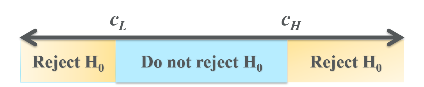
After choosing a test statistic $t_n$, the next step is to choose critical values. The critical values are two numbers $c_L$ and $c_H$ (where $c_L < c_H$) such that

$t_n$ has a high probability of being between $c_L$ and $c_H$ when the null is true.
$t_n$ has a lower probability of being between $c_L$ and $c_H$ when the alternative is true.

The range of values from $c_L$ to $c_H$ is called the critical range of our test.

Given the test statistic and critical values:

We reject the null if $t_n$ is outside of the critical range.
- This means we have strong evidence that $H_0$ is false.
- The reason we reject here is that we know we would be unlikely to observe such a value of $t_n$ if $H_0$ were true.
We fail to reject the null if $t_n$ is inside of the critical range.
- This means we do not have strong evidence that $H_0$ is false.
- This does not mean we have strong evidence that $H_0$ is true. We may just not have enough evidence to reach a conclusion.

Notice that there is an asymmetry here: in the absence of evidence, we will not reject any null hypotheses.

Critical values and rejecting the null hypothesis

How do we choose critical values? You can think of critical values as setting a standard of evidence, so we need to balance two considerations:

The probability of rejecting a false null is called the power of the test.
- We want our test to reject the null when it is false, so power is good.
The probability of rejecting a true null is called the size or significance of a test.
- We do not want our test to reject the null when it is true, so size is bad.
There is always a trade off between power and size
- A narrower critical range (higher $c_L$ or lower $c_H$) will increase the rejection rate, increasing both power (good) and size (bad).
- A wider critical range (lower $c_L$ or higher $c_H$) will reduce the rejection rate, reducing both power (bad) and size (good).

Given this trade off between power and size, we might construct some criterion that includes both (just like MSE includes both variance and bias) and choose critical values to maximize that criterion. In practice, we do not typically do that.

Instead, we follow a simple convention:

Set the size to a fixed value $\alpha$.
- In general, the conventional size varies by field, and typically varies with how much data is typical in that field.
- In economics and most other social sciences, the usual convention is to use a size of 5% ($\alpha = 0.05$).
- We sometimes see 1% ($\alpha = 0.01$) when working with larger data sets or 10% ($\alpha = 0.10$) when working with small data sets.
- In physics or genetics, where data sets are much larger, the conventional size is much lower.
Calculate critical values that imply the desired size.
- With a size of 5% $(\alpha = 0.05)$, we would:
  - set $c_L$ to the 2.5 percentile (0.025 quantile) of the null distribution
  - set $c_H$ to the 97.5 percentile (0.975 quantile) of the null distribution
- With a size of 10% $(\alpha = 0.10)$, we would:
  - set $c_L$ to the 5 percentile (0.05 quantile) of the null distribution
  - set $c_H$ to the 95 percentile (0.95 quantile) of the null distribution
- With a size of $\alpha$, we would:
  - set $c_L$ to the $\alpha/2$ quantile of the null distribution
  - set $c_H$ to the $1-\alpha/2$ quantile of the null distribution

In other words, we set size equal to a conventional value, and let the power be whatever is implied by that.

Example 8.5 Critical values for roulette

We earlier showed that the distribution of $t_n$ under the null is: \[t_n \sim Binomial(100,18/37)\] We can get a size of 5% by choosing: \[c_L = 2.5 \textrm{ percentile of } Binomial(100,18/37)\] \[c_H = 97.5 \textrm{ percentile of } Binomial(100,18/37)\] We can then use Excel or R to calculate these critical values. In Excel, the function you would use is BINOM.INV()

The formula to calculate $c_L$ is =BINOM.INV(100,18/37,0.025)
The formula to calculate $c_H$ is =BINOM.INV(100,18/37,0.975)

The calculations below were done in R:

## 2.5 percentile of binomial(100,18/37) = 39
## 97.5 percentile of binomial(100,18/37) = 58

In other words we reject the null (at 5% significance) that the roulette wheel is fair if red wins fewer than 39 games or more than 58 games.

A general test for a single probability

We can generalize the test we have constructed so far to the case of the probability of any event:

Test component	Roulette example	General case
Parameter	$p_{red} = \Pr(\textrm{Red wins})$	$p = \Pr(\textrm{event})$
Null hypothesis	$H_0:p_{red} = 18/37$	$H_0:p = p_0$
Alternative hypothesis	$H_1: p_{red} \neq 18/37$	$H_1: p \neq p_0$
Test statistic	$t = n\hat{f}_{RED}$	$t = n\hat{f}_{\textrm{event}}$
Null distribution	$Binomial(100,18/37)$	$Binomial(n,p_0)$
Critical value $c_L$	39	2.5 percentile of $Binomial(n,p_0)$
Critical value $c_H$	58	97.5 percentile of $Binomial(n,p_0)$
Decision	Reject if $t \notin [39,58]$	Reject if $t \notin [c_L,c_H]$

8.2.4 The power of a test

As mentioned above, the power of a test is defined as the probability of rejecting the null when it is false, and the alternative is true.

The size of a test is a number, since the distribution of the test statistic is known under the null. Since the alternative typically allows more than one value of the parameter $\theta$, the power of a test is not a number but a function of the unknown true value of $\theta$ (and sometimes other unknown features of the DGP): \[power(\theta) = \Pr(\textrm{reject $H_0$})\] In some cases we can actually calculate this function.

Example 8.6 The power curve for roulette

Power curves can be tricky to calculate, and I will not ask you to calculate them for this course. But they can be calculated, and it is useful to see what they look like.

Figure 8.1 below depicts the power curve for the roulette test we have just constructed; that is, we are testing the null that $p_{red} = 18/37$ at a 5% size. The blue line depicts the power curve for $n=100$ as in our example, while the green line depicts the power curve for $n=20$.

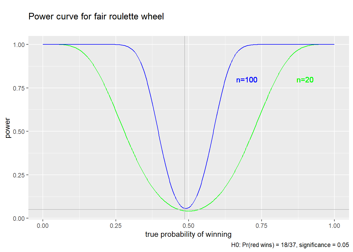
Figure 8.1: Power curves for the roulette example

There are a few features I would like you to notice, all of which are common to most regularly used tests:

The power curve reaches its lowest value at the red point $(18/37,0.05)$. Note that $18/37$ is the parameter value under the null, and $0.05$ is the size of the test. In other words:
- The power is always at least as big as the size, and is usually bigger.
- We are more likely to reject the null when it is false than when it is true. That’s good!
- When a test has this desirable property, we call it an unbiased test.
The power increases as $\theta$ gets further from the null.
- That is, we are more likely to detect unfairness in a game that is very unfair than when in one that is a little unfair.
Power also increases with the sample size; the blue line ($n = 100$) is above the green line ($n = 20$).

Power analysis is often used by researchers to determine how much data to collect. Each additional observation increases power but costs money, so it is important to spend enough to get clear results but not much more than that.

P values

The convention of always using a 5% significance level for hypothesis tests is somewhat arbitrary and has some negative unintended consequences:

Sometimes a test statistic falls just below or just above the critical value, and small changes in the analysis can change a result from reject to cannot-reject.
In many fields, unsophisticated researchers and journal editors misinterpret “cannot reject the null” as “the null is true.”

One common response to these issues is to report what is called the p-value of a test. The p-value of a test is defined as the significance level at which one would switch from rejecting to not-rejecting the null. For example:

If the p-value is 0.43 (43%) we would not reject the null at 10%, 5% or 1%.
If the p-value is 0.06 (6%) we would reject the null at 10% but not at 5% or 1%.
If the p-value is 0.02 (2%) we would reject the null at 10% and 5% but not at 1%.
If the p-value is 0.001 (0.1%) we would reject the null at 10%, 5%, and 1%.

The p-value of a test is simple to calculate from the test statistic and its distribution under the null. I won’t go through that calculation here.

8.3 The central limit theorem

In order for a test statistic to work, its exact probability distribution must be known under the null hypothesis. The example test in the previous section worked because it was based on a sample frequency, a statistic whose probability distribution is relatively easy to calculate. Unfortunately, most statistics do not have a probability distribution that is easy to calculate.

Fortunately, we have a very powerful asymptotic result called the Central Limit Theorem (CLT). The CLT roughly says that we can approximate the entire probability distribution of the sample average $\bar{x}_n$ by a normal distribution if the sample size is sufficiently large.

As with the LLN, we need to invest in some terminology before we can state the CLT. Let $s_n$ be a statistic calculated from $D_n$ and let $F_n(\cdot)$ be its CDF. We say that $s_n$ converges in distribution to a random variable $s$ with CDF $F(\cdot)$, or \[s_n \rightarrow^D s\] if \[\lim_{n \rightarrow \infty} |F_n(a) - F(a)| = 0\] for every $a \in \mathbb{R}$.

Convergence in distribution means we can approximate the actual CDF $F_n(\cdot)$ of $s_n$ with its limit $F(\cdot)$. As with most approximations, this is useful whenever $F_n(\cdot)$ is difficult to calculate and $F(\cdot)$ is easy to calculate.

CENTRAL LIMIT THEOREM: Let $\bar{x}_n$ be the sample average from a random sample of size $n$ on the random variable $x_i$ with mean $E(x_i) = \mu_x$ and variance $var(x_i) = \sigma_x^2$. Then \[z_n \rightarrow^D z \sim N(0,1)\]

What does the central limit theorem mean?

Fundamentally, it means that if $n$ is big enough then the probability distribution of $\bar{x}_n$ is approximately normal no matter what the original distribution of $x_i$ looks like.
In order for the CLT to apply, we need to re-scale $\bar{x}_n$ so that it has zero mean (by subtracting $E(\bar{x}_n) = \mu_x$) and constant variance as $n$ increases (by dividing by $sd(\bar{x}_n) = \sigma_x/\sqrt{n}$)). That re-scaled sample average is $z_n$.
In practice, we don’t usually know $\mu_x$ or $\sigma_x$ so we can’t calculate $z_n$ from data. Fortunately, there are some tricks for getting around this problem that we will talk about later.

What about statistics other than the sample average? Well it turns out that Slutsky’s theorem also extends to convergence in distribution.

SLUTSKY THEOREM: Let $g(\cdot)$ be a continuous function. Then: \[s_n \rightarrow^D s \implies g(s_n) \rightarrow^D g(s)\]

The implication here is that nearly all statistics have a sampling distribution that can be approximated using the normal distribution if the sample size is large enough.

8.4 Inference on the mean

Having described the general framework and a single example, we now move on to the most common application: constructing hypothesis tests and confidence intervals on the mean in a random sample.

Let $D = (x_1,\ldots,x_n)$ be a random sample of size $n$ on some random variable $x_i$ with unknown mean $E(x_i) = \mu_x$ and variance $var(x_i) = \sigma_x^2$.

Let the sample average be: \[\bar{x}_n = \frac{1}{n} \sum_{i=1}^n x_i\] let the sample variance be: \[s_x^2 = \frac{1}{n-1} \sum_{i=1}^n (x_i - \bar{x})^2\] and let the sample standard deviation be: \[s_x = \sqrt{s_x^2}\] These statistics are easily calculated from the data, and we have previously discussed their properties in detail.

8.4.1 The null and alternative hypotheses

Suppose that you want to test the null hypothesis: \[H_0: \mu_x = 1\] against the alternative hypothesis \[H_1: \mu_x \neq 1\] Having stated our null and alternative hypotheses, we need to construct a test statistic.

Remember that our test statistic needs to have a known distribution under the null, and a different distribution under the alternative.

8.4.2 The T statistic

The typical test statistic we use in this setting is called the T statistic, and takes the form: \[t_n = \frac{\bar{x}_n - 1}{s_x/\sqrt{n}}\] The idea here is that we take our estimate of the parameter ($\bar{x}$), subtract its expected value under the null ($1$), and divide by an estimate of its standard deviation ($s_x/\sqrt{n}$). We can add and subtract the unknown true mean $\mu_x$ to get: \[\begin{align} t_n &= \frac{\bar{x}_n - \mu_x + \mu_x - 1}{s_x/\sqrt{n}} \\ &= \frac{\bar{x}_n - \mu_x}{s_x/\sqrt{n}} + \frac{\mu_x - 1}{s_x/\sqrt{n}} \end{align}\] The first part of this expression is a random variable with a mean of zero and a variance of (about) one. The second part of the expression is exactly zero when $H_0$ is true, and not exactly zero when it is false.

Recall that we need the probability distribution of $t_n$ to be known when $H_0$ is true, and different when it is false. The second criterion is clearly met, and the first criterion is met if we can find the probability distribution of $\frac{\bar{x}_n - \mu_x}{s_x/\sqrt{n}}$.

Unfortunately, if we don’t know the exact probability distribution of $x_i$ we don’t know the exact probability distribution of statistics calculated from it. Once we have a potential test statistic, there are two standard solutions to this problem:

Assume a specific probability distribution (usually a normal distribution) for $x_i$. We can (or at least a professional statistician can) then mathematically derive the distribution of any test statistic from this distribution.
Use the central limit theorem to get an approximate probability distribution.

We will explore both of those options.

8.4.3 Asymptotic critical values

We will start with the asymptotic solution to the problem. As we learned in Chapter 7, the Central Limit Theorem tells us that: \[\frac{\bar{x}_n - \mu_x}{\sigma_x/\sqrt{n}} \rightarrow N(0,1)\] Under the null our test statistic looks just like this, but with the sample standard deviation $s_x$ in place of the population standard deviation $\sigma_x$. It turns out that Slutsky’s theorem allows us to make this substitution, and it can be proved that: \[\frac{\bar{x}_n - \mu_x}{s_x/\sqrt{n}} \rightarrow N(0,1)\]

Therefore, under the null: \[t_n \rightarrow N(0,1)\] In other words, while we do not know the exact (finite-sample) distribution of $t_n$ we know that $N(0,1)$ provides a useful asymptotic approximation to that distribution.

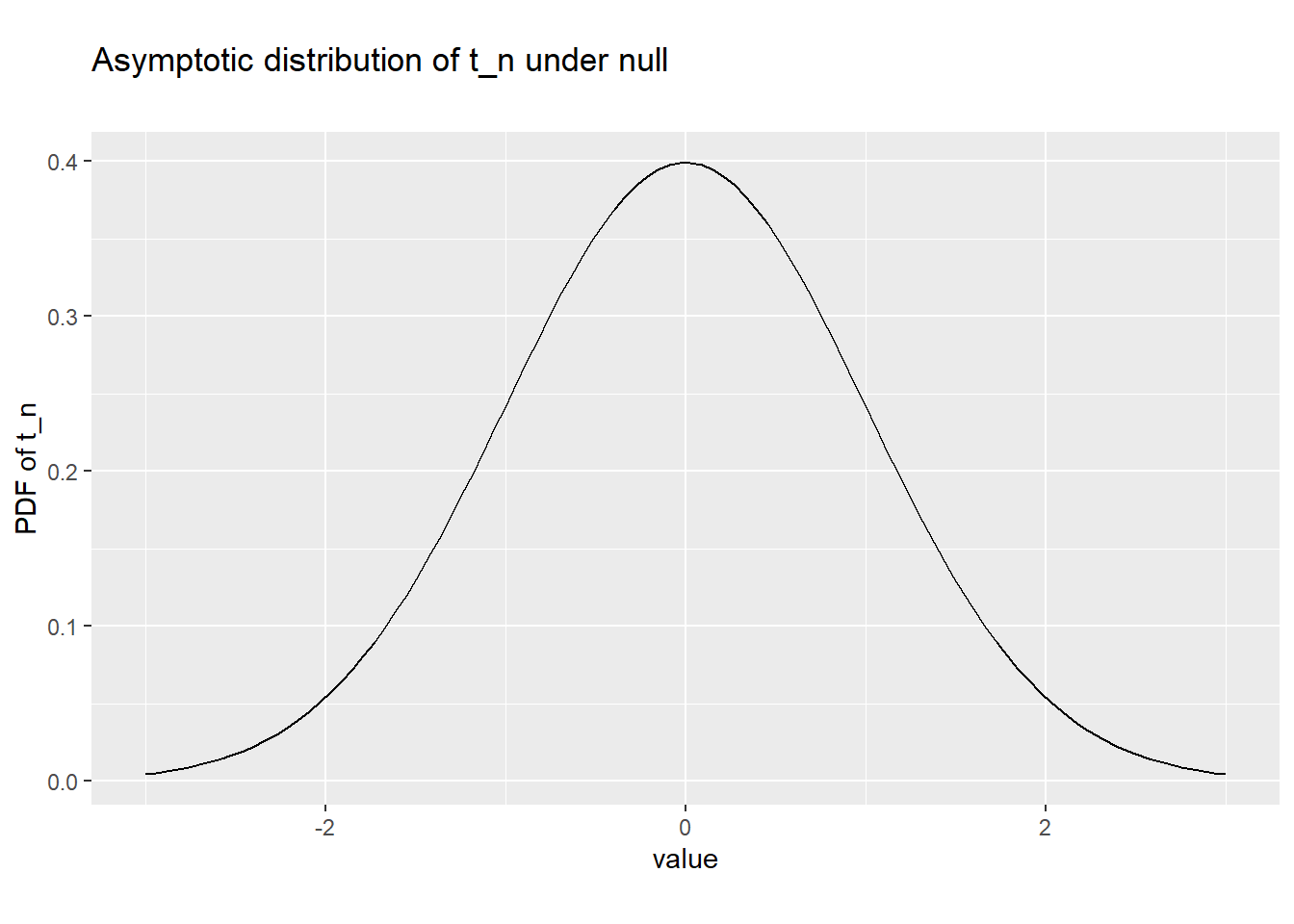
Figure 8.2: Asymptotic distribution of t_n under the null

Therefore, if we want a test that has the asymptotic size of 5%, we can use Excel or R to calculate critical values. In Excel, the function would be NORM.INV or NORM.S.INV, and the formulas would be:

$c_L$: =NORM.S.INV(0.025) or =NORM.INV(0.025,0,1).
$c_H$: =NORM.S.INV(0.975) or =NORM.INV(0.975,0,1).

The calculations below were done in R:

## cL = 2.5 percentile of N(0,1) =  -1.96
## cH = 97.5 percentile of N(0,1) =  1.96

These particular critical values are so commonly used that I want you to remember them.

8.4.4 Exact critical values

Most economic data comes in sufficiently large samples that the asymptotic distribution of $t_n$ is a reasonable approximation and the asymptotic test works well. But occasionally we have samples that are small enough that it doesn’t.

Another option is to assume that the $x_i$ variables are normally distributed: \[x_i \sim N(\mu_x,\sigma_x^2)\] where $\mu_x$ and $\sigma_x^2$ are unknown parameters.

Now at this point it is important to remind you: many interesting variables are not normally distributed (for example, our roulette outcome is discrete uniform, and the result of a given bet is Bernoulli) and so this assumption may very well be incorrect.

If this was a more advanced course I would derive the distribution of $t_n$ under the null. But for ECON 233, I will just ask you to understand that it can be derived once we assume normality of the $x_i$.

The null distribution of this particular test statistic under these particular assumptions was derived in the 1920’s by William Sealy Gosset, a statistician working at the Guinness brewery. To avoid getting in trouble at work (Guinness did not want to give away trade secrets) Gosset published under the pseudonym “Student.” As a result, the family of distributions he derived is called “Student’s T distribution.”

When the null is true, the test statistic $t_n$ as described above has Student’s T distribution with $n-1$ degrees of freedom: \[t_n \sim T_{n-1}\] As always, it has a different distribution (sometimes called the “noncentral T distribution”) when the null is false.

The $T_{n-1}$ distribution looks a lot like the $N(0,1)$ distribution, but has slightly higher probability of extreme positive or negative values. As $n$ increases the $T_{n-1}$ distribution converges to the $N(0,1)$ distribution, just as predicted by the central limit theorem.

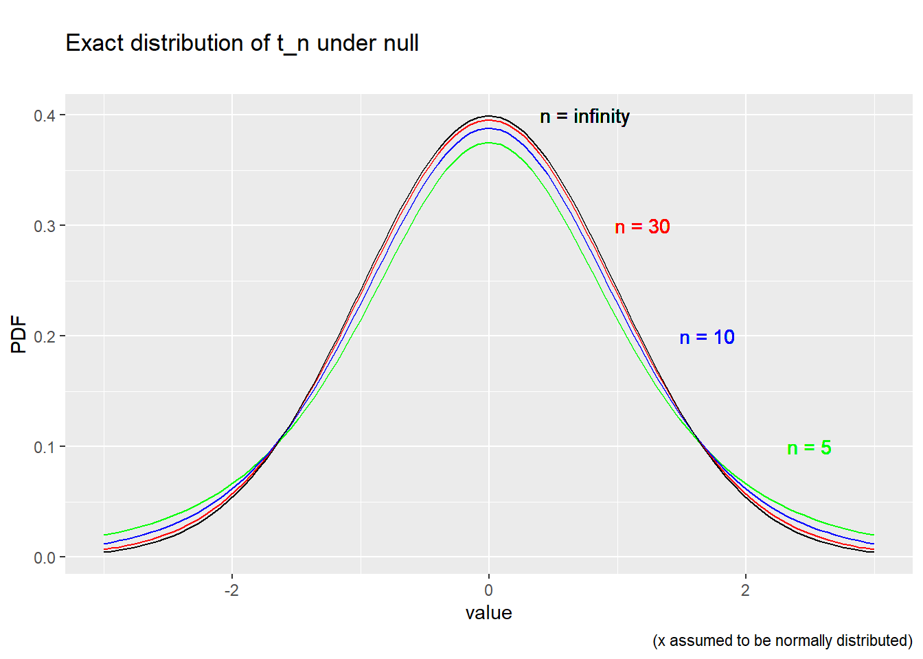
Figure 8.3: Exact distribution of t_n under the null

Having found our test statistic and its distribution under the null, we can calculate our critical values: \[c_L = 2.5 \textrm{ percentile of } T_{n-1}\] \[c_H = 97.5 \textrm{ percentile of } T_{n-1}\] We can obtain these percentiles using Excel or R. In Excel, the relevant function is T.INV. For example, if we have $n = 5$ observations, then:

We would calculate $c_L$ by the formula =T.INV(0.025,5-1).
We would calculate $c_H$ by the formula =T.INV(0.975,5-1).

The results (calculated below using R) would be:

## cL = 2.5 percentile of T_4 =  -2.776
## cH = 97.5 percentile of T_4 =  2.776

In contrast, if we have 30 observations, then:

We would calculate $c_L$ by the formula =T.INV(0.025,30-1).
We would calculate $c_H$ by the formula =T.INV(0.975,30-1).

The results (calculated below using R) would be:

## cL = 2.5 percentile of T_29 =  -2.045
## cH = 97.5 percentile of T_29 =  2.045

and if we have 1,000 observations:

We would calculate $c_L$ by the formula =T.INV(0.025,1000-1).
We would calculate $c_H$ by the formula =T.INV(0.975,1000-1).

The results (calculated below using R) would be:

## cL = 2.5 percentile of T_999 =  -1.962
## cH = 97.5 percentile of T_999 =  1.962

8.4.5 Which test to use?

Statisticians often call the finite-sample test the T test and the asymptotic test the Z test, as a result of the notation typically used to represent the test statistic. The two tests have the same underlying test statistic, but different critical values.

Which test should we use in practice? The T test is a more conservative test than the Z test, meaning it has larger critical values and is less likely to reject the null. As a result it has lower power and lower size. But at some point (around $n = 30$) the difference between the two tests becomes too small to make much of a difference.

As a result, statisticians typically recommend using the T test for smaller samples (less than 30 or so), and then using whichever test is more convenient with larger samples. Most data sets in economics have well over 30 observations so economists tend to use asymptotic tests unless they have a very small sample.

8.5 Confidence intervals

Hypothesis tests have one very important limitation: although they allow us to rule out $\theta = \theta_0$ for a single value of $\theta_0$, they say nothing about other values very close to $\theta_0$.

For example, suppose you are a medical researcher trying to measure the effect of a particular treatment, let $\theta$ be the treatment, and suppose that you have tested the null hypothesis that the treatment has no effect ($\theta = 0$).

If you reject this null, you have concluded that the effect has some effect. However, that does not rule out the possibility that the effect of the treatment is very small.
If you fail to reject this null, you cannot rule out the possibility that the treatment has no effect. However, this does not rule out the possibility that the effect is very large.

The solution to this would be to do a hypothesis test for every possible value of $\theta$, and classify them into values that were rejected and not rejected. This is the idea of a confidence interval.

A confidence interval for the parameter $\theta$ with coverage rate $CP$ is an interval with lower bound $CI_L$ and upper bound $CI_H$ constructed from the data in such a way that \[\Pr(CI_L < \theta < CI_H) = CP\] In economics and most other social sciences, the convention is to report confidence intervals with a coverage rate of 95%. \[\Pr(CI_L < \theta < CI_H) = 0.95\] Note that $\theta$ is a fixed (but unknown) parameter, while $CI_L$ and $CI_H$ are statistics calculated from the data.

How do we calculate confidence intervals? It turns out to be entirely straightforward: confidence intervals can be constructed by inverting hypothesis tests:

The 95% confidence interval is all values that cannot be rejected at a 5% level of significance.
The 90% confidence interval all values that cannot be rejected at a 10% level of significance.
- It is narrower than the 95% confidence interval.
The 99% confidence interval is all values that cannot be rejected at a 1% level of significance.
- It is wider than the 95% confidence interval.

Example 8.7 A confidence interval for the win probability

Calculating a confidence interval for $p_{red}$ is somewhat tricky to do by hand, but easy to do on a computer:

Construct a grid of many values between 0 and 1.
For each value $p_0$ in the grid, test the null hypothesis $H_0: p_{red} = p_0$ against the alternative hypothesis $H_1: p_{red} \neq p_0$.
The confidence interval is the range of values for $p_0$ that are not rejected.

For example, suppose that red wins on 40 of the 100 games. Then a 95% confidence interval for $p_{red}$ is:

## 0.32  to  0.49

Notice that the confidence interval includes the fair value of $0.486$ but it also includes some very unfair values. In other words, while we are unable to rule out the possibility that we have a fair game, the evidence that we have a fair game is not very strong.

8.5.1 Confidence intervals for the mean

Confidence intervals for the mean are very easy to calculate. Again we construct them by inverting the hypothesis test.

Pick any $\mu_0$. To test the null \[H_0: \mu_x = \mu_0\] our test statistic is: \[t_n = \sqrt{n}\frac{\bar{x}-\mu_0}{s_x}\] and we fail to reject the null if \[c_L < t_n < c_H\] where $c_L$ and $c_H$ are our critical values.

Plugging $t_n$ to this expression we fail to reject the null whenever: \[c_L < \sqrt{n}\frac{\bar{x}-\mu_0}{s_x} < c_H\] Solving for $\mu_0$ we fail to reject whenever: \[\bar{x} - c_H s_x/\sqrt{n} < \mu_0 < \bar{x} - c_L s_x/\sqrt{n}\] All that remains is to choose a confidence/size level, and decide whether to use an asymptotic or finite sample test.

If we are using the asymptotic approximation to construct a 95% confidence interval, then the 5% asymptotic critical values are $c_L = -1.96$ and $c_H \approx 1.96$ and the confidence interval is: \[CI = \bar{x} \pm 1.96 s_x/\sqrt{n}\] In other words, the 95% confidence interval for $\mu_x$ is just the point estimate plus or minus roughly 2 standard errors.

If we have a small sample, and choose to assume normality rather than using the asymptotic approximation, then we need to use the slightly larger critical values from the $T_{n-1}$ distribution. For example, if $n=5$, then $c_L \approx -2.78$, $c_H \approx 2.78$ and the 95% confidence interval is: \[CI = \bar{x} \pm 2.78 s_x/\sqrt{n}\] As with hypothesis tests, finite sample confidence intervals are typically more conservative (wider) than their asymptotic cousins, but the difference becomes negligible as the sample size increases.

Chapter review

In this chapter we have learned to formulate and test hypotheses, and to construct confidence intervals. The mechanics of doing so are complicated, but you should not let the various formulas distract you from the more basic idea of evidence: hypothesis testing is about how strong the evidence is in favor of (or against) a particular true/false statement about the data generating process, and confidence intervals are about finding a range of values for a parameter that are consistent with the observed data.

In practice, modern statistical packages automatically calculate and report confidence intervals for most estimates, and report the result of some basic hypothesis tests as well. When you need something more complicated, it is usually just a matter of looking up the command. I will ask you to do these calculations yourself so you get used to them, but it is more important that you can correctly interpret the results.

This is the last primarily theoretical chapter. The remaining chapters will be oriented towards data and applications.

Practice problems

Answers can be found in the appendix.

SKILL #1: Identify parameter, null and alternative

Suppose we have a research study of the effect of the minimum wage on employment. Let $\beta$ be the parameter defining that effect. Formally state a null hypothesis corresponding to the idea that the minimum wage has no effect on employment, and state the alternative hypothesis as well.

SKILL #2: Classify test statistics as valid or invalid

Which of the following characteristics do test statistics need to possess?
1. The distribution of the test statistic is known under the null.
2. The distribution of the test statistic is known under the alternative.
3. The test statistic has the same distribution whether the null is true or false.
4. The test statistic has a different distribution when the null is true versus when the null is false.
5. The test statistic needs to be a number that can be calculated from the data.
6. The test statistic needs to have a normal distribution.
7. The test statistic’s value depends on the true value of the parameter.

SKILL #3: Find distribution of test statistic under the null

Suppose we have a random sample of size $n$ on the random variable $x_i$ with unknown mean $\mu$ and unknown variance $\sigma^2$. The conventional T-statistic for the mean is defined as \[t = \frac{\bar{x}-\mu_0}{\hat{\sigma}_x/\sqrt{n}}\] where $\bar{x}$ is the sample average, $\mu_0$ is the value of $\mu$ under the null, and $\hat{\sigma}_x$ is the sample standard deviation.
1. What needs to be true in order for $t$ to have the $T_{n-1}$ distribution under the null?
2. What is the asymptotic distribution of $t$?

SKILL #4: Describe distribution of test statistic under the alternative

Consider the setting from problem 3 above, and suppose that the true value of $\mu$ is some number $\mu_1 \neq \mu_0$. Write an expression describing $t$ as the sum of (a) a random variable that has the $T_{n-1}$ distribution and (b) a random variable that is proportional to $\mu_1-\mu_0$.

SKILL #5: Find the size of a test

Suppose that we have a random sample of size $n=14$ on the random variable $x_i \sim N(\mu,\sigma^2)$. We wish to test the null hypothesis $H_0: \mu = 0$. Suppose we use the standard t-statistic: \[t = \frac{\bar{x}-\mu_0}{\hat{\sigma}_x/\sqrt{n}}\]
1. Suppose we use critical values $c_L = -1.96$ and $c_H = 1.96$. Use Excel to calculate the exact size of this test.
2. Suppose we use critical values $c_L = -1.96$ and $c_H = 1.96$. Use Excel to calculate the asymptotic size of this test.
3. Suppose we use critical values $c_L = -3$ and $c_H = 2$. Use Excel to calculate the exact size of this test.
4. Suppose we use critical values $c_L = -3$ and $c_H = 2$. Use Excel to calculate the asymptotic size of this test.
5. Suppose we use critical values $c_L = -\infty$ and $c_H = 1.96$. Use Excel to calculate the exact size of this test.
6. Suppose we use critical values $c_L = -\infty$ and $c_H = 1.96$. Use Excel to calculate the asymptotic size of this test.

SKILL #6: Find critical values

Suppose that we have a random sample of size $n=18$ on the random variable $x_i \sim N(\mu,\sigma^2)$. We wish to test the null hypothesis $H_0: \mu = 0$. Suppose we use the standard t-statistic: \[t = \frac{\bar{x}-\mu_0}{\hat{\sigma}_x/\sqrt{n}}\]
1. Use Excel to calculate the (two-tailed) critical values that produce an exact size of 1%.
2. Use Excel to calculate the (two-tailed) critical values that produce an exact size of 5%.
3. Use Excel to calculate the (two-tailed) critical values that produce an exact size of 10%.
4. Use Excel to calculate the (two-tailed) critical values that produce an asymptotic size of 1%.
5. Use Excel to calculate the (two-tailed) critical values that produce an asymptotic size of 5%.
6. Use Excel to calculate the (two-tailed) critical values that produce an asymptotic size of 10%.

SKILL #7: Construct and interpret a confidence interval

Suppose we have a random sample of size $n = 16$ on the random variable $x_i \sim N(\mu,\sigma^2)$, and we calculate the sample average $\bar{x} = 4$ and the sample standard deviation $\hat{\sigma} = 0.3$.
1. Use Excel to calculate the 95% (exact) confidence interval for $\mu$.
2. Use Excel to calculate the 90% (exact) confidence interval for $\mu$.
3. Use Excel to calculate the 99% (exact) confidence interval for $\mu$.
4. Use Excel to calculate the 95% asymptotic confidence interval for $\mu$.
5. Use Excel to calculate the 90% asymptotic confidence interval for $\mu$.
6. Use Excel to calculate the 99% asymptotic confidence interval for $\mu$.

SKILL #8: Interpret test results and confidence intervals

Suppose you estimate the effect of a university degree on earnings at age 30, and you test the null hypothesis that this effect is zero. You conduct a test at the 5% level of significance, and reject the null. Based on this information, classify each of these statements as “probably true,” ’possibly true“, or”probably false":
1. A university degree has no effect on earnings.
2. A university degree has some effect on earnings.
3. A university degree has a large effect on earnings.
Suppose you estimate the effect of a university degree on earnings at age 30, and you test the null hypothesis that this effect is zero. You conduct a test at the 5% level of significance, and fail to reject the null. Based on this information, classify each of these statements as “probably true,” ’possibly true“, or”probably false":
1. A university degree has no effect on earnings.
2. A university degree has some effect on earnings.
3. A university degree has a large effect on earnings.
Suppose you estimate the effect of a university degree on earnings at age 30, and your 95% confidence interval for the effect is $(0.10,0.40)$, where an effect of 0.10 means a degree increases earnings by 10% and an effect of 0.40 means that a degree increases earnings by 40%. Based on this information, classify each of these statements as “probably true,” ’possibly true“, or”probably false":
1. A university degree has no effect on earnings.
2. A university degree has some effect on earnings.
3. A university degree has a large effect on earnings, where “large” means at least 10%.
4. A university degree has a very large effect on earnings, where “very large” means at least 50%.

Test component	Roulette example	General case
Parameter	\(p_{red} = \Pr(\textrm{Red wins})\)	\(p = \Pr(\textrm{event})\)
Null hypothesis	\(H_0:p_{red} = 18/37\)	\(H_0:p = p_0\)
Alternative hypothesis	\(H_1: p_{red} \neq 18/37\)	\(H_1: p \neq p_0\)
Test statistic	\(t = n\hat{f}_{RED}\)	\(t = n\hat{f}_{\textrm{event}}\)
Null distribution	\(Binomial(100,18/37)\)	\(Binomial(n,p_0)\)
Critical value \(c_L\)	39	2.5 percentile of \(Binomial(n,p_0)\)
Critical value \(c_H\)	58	97.5 percentile of \(Binomial(n,p_0)\)
Decision	Reject if \(t \notin [39,58]\)	Reject if \(t \notin [c_L,c_H]\)