Chapter 2 Basic data cleaning with Excel
Before we can analyze data, we usually need to clean it. Cleaning data means putting it into a form that is ready to analyze, and can include:
- Converting data files from one file format to another
- Reorganizing complex tables of data into simple tables
- Combining data from multiple tables into a single table
- Modifying existing variables
- Creating new variables
In this course, we will do most of our data cleaning using Excel.
This chapter will develop both both some principles of data cleaning and the basic Excel tools needed to implement them . We will also apply this knowledge by using Excel to clean a real data set.
Chapter goals
In this chapter we will learn how to:
- Use basic Excel terminology and concepts including:
- Workbooks, worksheets, and cells
- Cell contents and display format
- Cell ranges
- Relative and absolute cell addresses
- Numeric, text, date, and logical data types
- Use Excel tools to view data, including:
- Sorting
- Filtering
- Freezing panes
- Changing cell size
- Use Excel tools to enter new data and “clean” existing data, including
- Fill and series
- Formulas
- Functions
- Number formats
- Follow good data management practices
- Practice data documentation and version control
- Identify the characteristics of tidy data
2.1 Application: Canadian employment data
We will demonstrate the key principles and tools in this chapter
by cleaning the November 2020 employment data for Canadian provinces. The
data can be found in the file
https://bookdown.org/bkrauth/BOOK/sampledata/CanEmpNov20.xlsx
Economics review: Employment statistics
Employment statistics are typically covered in a Principles of Macroeconomics course (at SFU, this course is called ECON 105). To review the basics:
- These statistics are reported monthly by Statistics Canada and
are based on the Labour Force Survey (LFS), a monthly survey of the
civilian, non-institutionalized, working-age population of Canada.
- “civilian” excludes those on active military duty
- “non-institutionalized” excludes people in prison, hospitals, nursing homes, etc.
- “working-age” excludes those under age 15
- People living on reserve are also not covered by the LFS
- The LFS population is grouped into three categories:
- Employed: worked for pay or profit in the previous week, or had a job and was absent (e.g. due to illness or vacation).
- Unemployed: not employed in the previous week, but either looking for work, on temporary layoff, or had a job to start within the next four weeks.
- Not in the labour force: everyone else. This includes retirees, full-time students who aren’t working for pay, and anyone else who is neither working nor looking for work.
- These basic counts are then used to calculate several other statistics
- The labour force is the total count of those who are employed or unemployed.
- The labour force participation rate is the proportion or percentage of the population that is in the labour force. The Canadian LFP rate is typically around 65%.
- The unemployment rate is the proportion of the labour force that is unemployed. The Canadian unemployment rate is typically 5-10%.
The unemployment rate and LFP rate are key indicators of labour market conditions. A higher-than-usual unemployment rate means that workers are having difficulty finding work, and a lower-than-usual LPF rate means that some workers have stopped looking for work.
2.2 Data cleaning principles
Next, we describe some of the core principles we will follow in cleaning and managing our data.
2.2.1 Reproducibility
When analyzing data it is important for the results of our analysis to be reproducible. What that means is that an interested reader should be able to figure out exactly how you got your results, and should be able to generate those results themselves. Note that the “interested reader” might be you, as it is common to return to an analysis you did earlier. Without reproducibility, you may not remember where you found the data, what you have done with it, or what it means.
Reproducibility requires that we treat our data with care. In particular, we should:
- Document the original sources for all data.
- If a data file is downloaded from the internet, the original URL should be documented.
- Keep an unmodified copy of all original data.
- Avoid directly editing data. Add new data instead.
- Sometimes this is not possible or practical, which is why we keep an unmodified copy of the original data.
- Give all files and variables brief but informative names.
- Avoid spaces or special characters in variable or file names. They can cause problems when moving data between operating systems, file formats, or applications.
We will discuss the implementation of these principles later in this chapter.
2.2.2 Tidy data
To keep analysis easy and minimize errors, data should be organized as what data scientists have come to call tidy data. Tidy data has the following seven properties:
- Data is arranged in one or more simple rectangular grids or tables.
- Each column in a table represents a distinct variable or attribute.
- Each variable has an informative and unique variable name.
- Variable names are typically displayed in the top row of the table.
- Each row in a table (after the top row) represents a distinct observation, data point or case.
- All observations in a given table come from the same
unit of observation
- For example, data on Canadian cities and data on Canadian provinces should probably be in two separate tables.
- One variable in a table serves as a unique identifier or ID for the
observation.
- A unique identifier takes on a different value for each observation.
- The ID variable is often in the first column of the table.
- The order in which observations or variables are listed is irrelevant to
the analysis.
- That is, the interpretation of the table would not change if its rows or columns were in a different order.
Data that is not tidy is sometimes called messy data. One of the first steps in cleaning data is rearranging it from a messy format to a tidy format.
2.2.3 Observations and identifiers
Each tidy data set normally includes at least one unique identifier or ID variable. By definition, an ID variable must take on a different value for each observation. With this property, we can use ID variables to link and combine data from multiple sources.
Example 2.1 ID variables at SFU
SFU is one of British Columbia’s largest organizations, and relies heavily on ID variables to organize its information:
- Each person at SFU (faculty, staff or student) has a unique 16-digit ID number and a unique computing ID.
- Each semester at SFU has a 4-digit semester code. For example, Fall 2021 is assigned the semester code 1217.
- Each academic program at SFU has a 2-letter to 4-letter program code such as IS, BUS, or ECON.
- Each course at SFU is uniquely identified by the combination of its program code (e.g. ECON) its numeric course code (e.g. 233), its section number (e.g., D100), and its semester number (e.g., 1217).
Your library records, grades, financial records, and almost any other information SFU has about you includes one or more of these IDs.
The example above shows several common characteristics of ID variables:
- They can be numbers (like your student ID number) or text strings (like your computing ID).
- They can be
- Assigned sequentially or arbitrarily (like your student ID number),
- Constructed by a formula (like semester codes).
- Standardized and listed in a table (like program codes)
- An observation can sometimes be identified by combining identifiers. For example, a specific course at SFU might be “ECON233-D100-1217.”
ID variables should ideally be portable across applications and systems. That is, our ID variable should still work if we move data from a Windows PC to a Linux or Apple system, and should still work if we move from Excel to R or Python. To maximize portability, keep in mind the following potential issues:
| Issue | Solution |
|---|---|
| Some applications will round non-integer values (changing 1.23 to 1) or drop leading zeros (changing 00045 to 45). | Numeric ID variables should always be integers without leading zeros, or converted to text. |
| Some applications will reject or transform spaces or unusual characters. | Text ID variables should only use (Latin) letters and (Arabic) digits. |
| Some applications are case-sensitive (so that “hello” and “Hello” are different values) and others are not. | Text ID variables should typically use either all upper-case or all lower-case. |
It’s OK for an ID variable to be nearly-but-not-exactly identical to some other variable. For example a Canadian data set might have both a Province variable that takes on values like “Québec” and “Nova Scotia” and a ProvinceID variable that takes on values like “QUEBEC” and “NOVASCOTIA.”
Names, IDs, and probabilistic matching
Proper names are typically not used as ID variables since they are not necessarily unique. In addition, they are not always written consistently. For example, the same person might be called “Doug” in one data set and “Douglas” in another.
Occasionally a data set will not have a standardized ID variable, and our only option is to match observations based on a proper name. For example, in BC school data an ID number called a PEN while health data uses a different ID number called a PHN. There is no direct way to match PEN and PHN, so we have to match education and health records on a combination of proper names and other information such as year of birth. Matches made this way are called “probabilistic” matches, meaning (roughly) that the records probably describe the same person but might not.
2.3 Introduction to Excel
Excel is the most commonly-used example of a spreadsheet, a software program designed for the tabulation, analysis, and display of data. Its main competitors include Google Sheets and Apple Numbers. It is widely used in business and government, so good Excel skills are valuable in the labour market.
Many of you have probably used Excel before, but there are many features you are probably not yet familiar with. We will start by going over some of its basic characteristics and terminology.
2.3.1 Terminology and interface
Start Excel. Your screen should look something like this:
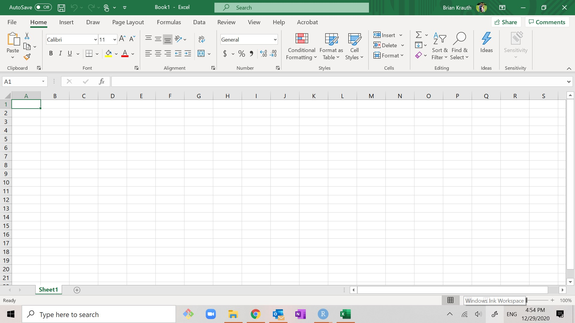
When giving instructions, I will refer to various elements of Excel’s user interface by name. You may have been using these elements for years without ever knowing their names, so I will list them here:
- The menu bar is at the top of the screen:

- The ribbon is below the menu bar

- The ribbon has buttons for performing simple actions.
- The buttons are grouped by function, for example the ribbon above
depicts groups called
Clipboard,Font, etc.- Within each function group, there is usually a little
 icon in the lower-right corner that you can click on to access
additional options.
icon in the lower-right corner that you can click on to access
additional options.
- Within each function group, there is usually a little
- If your ribbon is not visible:
- You can make it visible by selecting
Home(or anything else) on the menu bar. - Once you have made the ribbon visible, you can keep it visible by clicking on the little thumbtack icon in its lower right corner.
- You can make it visible by selecting
- The contents of the ribbon depend on the currently-active menu bar option
(usually but not always
Home).- I will assume that
Homeis the currently-active option; if it isn’t you can just selectHometo make it the currently-active option.
- I will assume that
- The formula bar is just below the ribbon.

- It shows the contents of the current cell.
- You can type in it to change the contents of the current cell.
- The insert function button is to the left of the formula bar.

- We will learn to use this later.
- Most of the screen displays a grid of cells that is called
a spreadsheet or worksheet:
- Columns are identified by letter.
- Rows are identified by number.
- Cells are identified by column and row. For example, the cell in column A, row 2 is called cell A2.
- Below the worksheet is a row of tabs:

- You can click on a tab to switch to that worksheet.
- You can double-click on a tab to change its name.
- You can click on the “+” button to add a new worksheet.
- An Excel file is called a workbook.
- Each workbook contains one or more worksheets.
- in Windows, Excel files normally have the
.xlsxextension. - Older files sometimes have the
.xlsextension.
2.3.2 Viewing data
The first step in any data cleaning exercise is to look at the data and assess what needs to be done.
Example 2.2 Overview of the employment data
Open the data file in Excel. As you can see, this Excel workbook contains three worksheets:
- Employment Nov 2020 is our main data table:
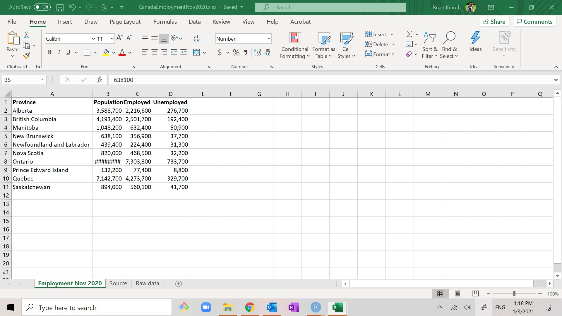 It is in tidy format:
- There is a single rectangular table starting in cell A1.
- Each row represents a Canadian province
- Canadian provinces are the unit of observation
- Each column represents a variable describing that province
- The top row shows brief but clear names for each variable
- The provinces are listed in alphabetical order, but the interpretation of the table would not change if they were listed in some other order
- Raw data is the original data as downloaded from Statistics
Canada.
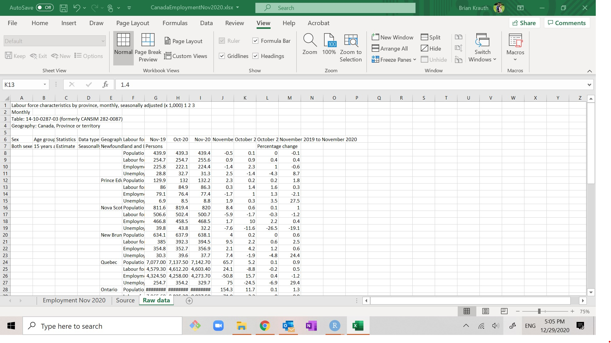 It is messy (the opposite of tidy)
- The table starts in cell A6 rather than cell A1.
- Variables (Population, Labour Force, etc.) are in rows rather than columns.
- Observations (the unit of observation is the province-month) are in both rows and columns.
- Cells are filled in “implicitly.” For example, there is nothing in row 17 that says what province it describes, but we know that it describes Nova Scotia because it comes after row 16 (which does say it describes Nova Scotia). As a result, the order of rows is very important.
- Source describes where the original data was obtained.
Note that we are following good data management practice by saving a copy of the original data and creating a new data set based on it, rather than by directly editing the original data. We are also documenting data sources. Both of these practices will enhance the reproducibility and reliability of our analysis.
In the remainder of this section, we will learn a few tools for changing how our data is displayed that do not change the content of the data.
2.3.3 Sorting, filtering, and freezing
Sorting allows us to re-order the rows of our data based on the value in one or more of the columns. Since order does not matter with tidy data, we can sort in whatever way we like without changing the content of our data.
Example 2.3 Sorting the employment data
The original data are in alphabetical order by province name. But suppose we wanted it to be ordered by population (with the highest populations on top) instead. Here’s all we need to do:
- Select any cell in the Population column.
- Select
Home > Sort and Filter > Sort Largest to Smallest.
As you can see, the data set is now sorted by population. We can follow similar steps to put the data set back in alphabetical order:
- Select any cell in the Province column.
- Select
Home > Sort and Filter > Sort A to Z.
Notice that Excel can tell whether a column contains numbers or text, and will sort accordingly.
You can sort in ascending or descending order, and you can sort on multiple columns by selecting the “Custom sort” option.
Filtering allows us to hide some observations so we can look at a particular subset of observations that we are interested in. The hidden observations are still there.
Example 2.4 Filtering the employment data
Suppose we only want to see data for larger provinces. Here’s what we can do:
- Select
Home > Sort and Filter > Filter. If you look at the column headers in your sheet you will see that they have become drop-down boxes. - Click on the drop-down box for Population, then select
Number filters > Greater Than... - Enter one million (
1000000) in the box and selectOK.
At this point, only the provinces with at least one million residents appear in the table. Don’t worry, the other ones haven’t gone anywhere.
We can undo the filter and remove the drop-down boxes by selecting
Home > Sort and Filter > Filter again.
You can filter on more complex criteria, and you can combine sorting and filtering.
Freezing panes keeps some rows and/or columns visible regardless of which cell is currently selected. This allows us to work with large tables while keeping the top row (variable names) and/or the first column (observation IDs) visible.
Example 2.5 Freezing panes
Go down to row 50 or so in your worksheet. Notice that you can’t see the variable names in row 1 any more. This is fine for our current data set, but it would be a problem if we had more than a few rows.
- Go back to cell A1.
- Select
View > Freeze Panes > Freeze Top Row.
Now go back down to row 50 or so. You will see that the top row is still displayed and you can see the variable names.
To undo this, select View > Freeze Panes > Unfreeze Panes.
Instead of freezing the first row, you can freeze the first column, or you can freeze any number of rows and columns.
2.3.4 Cell formatting
Another way we can change the appearance of our data without changing its content is to adjust the cell formatting for one or more cells. Cell formatting characteristics include:
- Column width
- Row height
- Font
- Bold/italics/underline
- Text color
- Background color
- Cell borders
- Alignment (left/right/center as well as top/bottom/middle)
The procedure for modifying the cell format is straightforward if you regularly use productivity applications like Microsoft Word.
Example 2.6 Changing cell size
You may notice that cell B8 (Ontario population) appears to contain “######” rather than a number. The cause of this problem is that the cell is not wide enough to display the correct number. So let’s make it wider.
We have several options for doing this:
- From the menu: Select any cell in column B, and then select
Home > Format > Cell Width.... A dialog box will appear that allows you to enter your preferred width. Try 10. - With the mouse: Move your cursor to the line between column headers B
and C until the cursor looks like this:
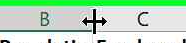 . Click on the mouse and drag the cursor to
resize the column.
. Click on the mouse and drag the cursor to
resize the column. - Auto-fit (this is what I usually do): Move your cursor to the line between column headers B and C, and double-click. The column width will automatically adjust to fit the data.
You can follow similar procedures to adjust the row height.
Another important cell formatting characteristic is the number format, which will be discussed in a later section.
2.4 Cleaning data
We are now ready to start actively cleaning our data.
2.4.1 Preparation
We start by making two copies of our data set:
- The original file, exactly as we received it.
- A working copy under a new name.
Recall that one of our core principles of reproducibility is to always keep an unmodified copy of the original data. We will do any modifications or additions in the working copy.
Example 2.7 Creating a working copy
Save your Excel workbook, giving it a different name from the name of the original data file.
As we proceed through the example application, be sure to save your working copy each time you make a significant modification or addition.
The next step is to look at the data and construct a cleaning plan. Your cleaning plan should have several steps:
- Convert all data into tidy-format tables.
- Ensure that each table has a unique ID variable.
- Identify and address problems in existing variables.
- Create new variables that may be useful.
- Link data across tables.
The data cleaning plan should be based around what we plan to do with the data, but should preserve flexibility in case we want to use the data for other purposes.
Example 2.8 A plan for cleaning the employment data
The first step in cleaning the employment data is to ensure we have tidy data. This step has already been completed, so we can move on.
The second step is to ensure that each table has a unique ID variable. In our employment data, the province name could serve as a unique identifier, but names typically have some drawbacks:
- Names are not always unique. This is obviously not an issue with Canadian provinces, but it is an issue in many other data sets. For example, there are 41 cities and towns in the United States named “Springfield.”
- The same observation often appears with different names in different data sets. For example, some older data sets call the province of Newfoundland and Labrador just “Newfoundland” as that was the province’s name before December 6, 2001.
As a result, it is typically not advisable to use names as ID variables. Instead, we could:
- Use a standardized code such as the two-letter postal abbreviation.
- Assign an arbitrary number to each observation.
We will do both.
The third step is to identify and address problems in our existing variables.
The fourth step is to consider is whether there are any variables we would like to analyze that have not yet been constructed. In our employment data, we will want to construct
- Labour force
- Labour force participation rate
- Unemployment rate
We will also want to include information on which specific month these observations are describing (November 2020). Although that information is in the Raw data worksheet and in the title of the main worksheet (Employment Nov 2020) it may be useful to have it in the table as well.
We will now add several variables to our working data set. Be sure to save the file after adding each variable so that you don’t lose your work.
2.4.2 Inserting cells
Most of the time we will add data to the end of the existing table, adding new variables after the last column or new observations after the last row. But occasionally we will want to insert a column or row into our table.
Example 2.9 Adding a column for the ID variable
We will want our first column to include a not-yet-constructed ID variable, so we need to insert a column to the left.
- Select any cell in column A.
- Select
Home > Insert > Insert Sheet Columnsfrom the menu.
This will shift all columns to the right, and insert a new blank column A.
We can also insert rows, delete rows or columns, and even insert or delete individual cells.
2.4.3 Data entry, fill and series
The simplest way to add a variable to an Excel table is by typing data directly into the cells.
Example 2.10 Entering data
As we discussed earlier, we would like to add the two-letter postal abbreviation for each province:
| Province or Territory | ProvAbb |
|---|---|
| Alberta | AB |
| British Columbia | BC |
| Manitoba | MB |
| New Brunswick | NB |
| Newfoundland and Labrador | NL |
| Northwest Territories | NT |
| Nova Scotia | NS |
| Nunavut | NU |
| Ontario | ON |
| Prince Edward Island | PE |
| Quebec | QC |
| Saskatchewan | SK |
| Yukon | YT |
The postal abbreviation is useful for at least two reasons
- It is standardized, while the full province name may not be.
- Quebec is sometimes written Québec.
- It is short, which can be useful in charts.
To add this variable:
- Enter ProvAbb in cell F1 to name the variable.
- Fill in cells F2:F11 with the correct postal abbreviation.
Excel has several tools available to speed the process of entering data. First, you can copy-and-paste or cut-and-paste the contents of any cell into any other cell.
Excel’s fill tool allows you to quickly copy the contents of a cell into a set of cells immediately, above, below or to the left or right.
Example 2.11 Using fill
Our data cleaning plan includes adding a variable indicating which month and year these particular observations describe (November 2020).
- Enter MonthYr in cell G1 to name the variable.
- Enter “11/20” in cell G2.
- You may notice that Excel displays the date differently from
how you entered it - on my computer it displays as
Nov-20. We will talk more later about how Excel handles dates.
- You may notice that Excel displays the date differently from
how you entered it - on my computer it displays as
Now we could enter the exact same date in cells G3:G11, but we can save ourselves some time by using Excel’s fill tool:
- Select cells G2:G11.
- Select
Home > Fill > Down.
As you can see, Excel fills in all selected cells with the value in the top cell.
The series tool allows you to fill in a group of cells with an ascending or descending sequence of numbers or dates.
Example 2.12 Using series
Let’s create a unique sequential ID variable in column A. We can enter these ID numbers by hand, but there is an easier way using Excel’s series tool:
- Enter ID in cell A1 to name the variable.
- Enter 1 in cell A2.
- Select cells A2:A11.
- Select
Fill > Series.... The Series dialog box will appear. - There are several options for constructing a series. Fortunately, the
default is exactly what we want, so select
OK.
As you can see, column A now contains a unique identifier that numbers provinces from 1 to 10.
2.4.4 Formulas
Most of our new variables will be calculated from existing variables using formulas. A formula is just a rule for calculating a value from some other values.
Formulas always start with the equals sign = followed by a mathematical
expression that can include any combination of:
- Specific values, for example
=2or=TRUE - References to other cells, for example
=D2 - Standard arithmetic operators, for example
=2+2or=D2/4 - Functions, for example
=SQRT(D2)or=SUM(D2:D10).
Formulas can be simple, or they can be quite complex.
Example 2.13 Calculating the labour force
Returning to our application, everyone who is either employed or unemployed is in what economists call the “labour force.” So let’s add that variable.
- Enter LabourForce in cell H1 to name the variable.
- Note that I avoid putting spaces in variable names. This is a habit of mine when working with data, because spaces can cause complications when moving data across systems, e.g. from Excel to R.
- Enter
= D2 + E2in cell H2.
Cell H2 now displays 2,493,300 which is in fact the value in cell D2
plus the value in cell E2.
As discussed earlier, it is important to distinguish between what is
the contents of a cell and how those contents are displayed. For
example, the true contents of cell H2 in our example above are the
formula = D2 + E2 but the cell shows the number 2,493,300. If
you change the number in cell D2 or cell E2, the number shown in
cell H2 will adjust accordingly.
Formulas can use the results from other formulas, as shown in the example below.
Example 2.14 Calculating unemployment and LFP rates
Let’s add a column for the labour force participation rate. To remind you, this is the proportion or percentage of the population (column C) that is in the labour force (column H).
- Enter LFPRate in cell I1 to name the variable.
- Enter
=H2/C2in cell I2 to calculate the variable.
Let’s also add a column for the unemployment rate. To remind you, this is the proportion or percentage of the labour force (column H) that is unemployed (column E).
- Enter UnempRate in cell J1 to name the variable.
- Enter
=E2/H2in cell J2 to calculate the variable.
Notice that both of these formulas use cell H2, which itself contains a formula.
2.4.5 Functions
Excel has about 500 built-in functions that we can use in formulas. Each function has a name and a set of arguments whose values you can set.
To use a function, you simply include its name and its arguments as
part of the formula. For example, the SQRT() function takes a single
numeric argument and returns the square root of the argument. So if
you enter =SQRT(2) in a cell, the cell will display 1.414, the
square root of 2.
Excel also has extensive tools for
- Finding the function you need for a particular calculation task.
- Figuring out what arguments to use in the function.
You can also use Google or any other search engine to find this information.
Example 2.15 A simple function
Suppose we want to add a new variable for the (natural) log of population.
- Enter LogPop in cell K1 to give the variable a name.
- Select cell K2.
- If we already know the name of the function for taking the natural
log, we can just type in our formula. But suppose we don’t know
the name of the function, or even whether there is such a function.
- Click on the insert function button
to the left of the formula bar.
- The
Insert Functiondialog box will appear. It will have a very long list of functions. You will want to narrow this list down, and you have several options for doing so:- Search: Enter
logarithmin theSearch for a functiontext box. - Browse: Select
Math & Trigfrom theOr select a categorydrop-down box.
- Search: Enter
- Once you have narrowed the list down, it is easy to find the
function you want (
LN). SelectLNfrom theSelect a functionlist box, and then selectOK.You will now see theFunction Argumentsdialog box for theLNfunction.
- Click on the insert function button
- As you can see, the
LNfunction takes one argument (the number you want the log of). You want to take the log of cell C2, so enter the textC2here or click on cell C2.- the dialog box will display the value in cell C2 (
3588700) as well as the calculated value for the log of cell C2 (15.0933058).
- the dialog box will display the value in cell C2 (
- Select
OK.
You will see that cell K2 now contains =LN(C2) which displays as 15.0933.
Note that if you already knew the function and arguments you needed, you could
have just typed =LN(C2) into cell K2 instead.
2.4.6 Cell ranges
Some functions like SUM() and AVERAGE() operate on a range of cells
rather than a single cell. A range is just a rectangular set of cells,
and is described by its upper-left and lower-right cells, separated
by a colon (“:”). For example:
- Range A2:A5 consists of cells A2, A3, A4 and A5.
- Range A2:C2 consists of cells A2, B2, and C2.
- Range A2:B3 consists of cells A2, B2, A3, and C3.
A single cell can also be thought of as a range of cells with one row and one column.
Example 2.16 Total population
Suppose we want to create a new variable that reports the total population
across all observations in the data. The function to do that is SUM().
- Enter TotPop in cell L1 to give the variable a name,
- Enter
=SUM(C2:C11)in cell L2.
Cell L2 should display 31,275,600 which is indeed the sum of
cells C2 to C11.
2.4.7 Copying formulas
In Excel, you can copy-and-paste the contents of a cell to any other cell. This is particularly handy when a cell contains a formula, as it would be inconvenient to type the same formula into each cell.
Example 2.17 Copying a formula
To use copy-and-paste to copy the formula in cell H2 to the other cells in column H:
- Select cell H2 and copy it.
- Select cells H3:H11 and paste.
You can also use fill for this purpose, and it is usually quicker.
Example 2.18 Filling a formula
To use fill to copy the formulas in cells I2:L2 to the other cells in columns I through L:
- Select cells I2:L11
- Select
Home > Fill > Down
2.4.8 Relative and absolute references
Excel is smart and normally treats cell addresses in formulas as relative references when copying and pasting cells. That is, when a formula is copied to another cell \(a\) columns to the right and \(b\) rows down, the column letters in the formula are increased by \(a\) units, and the row numbers are increased by \(b\) units.
For example, suppose cell B5 contains the formula =A1. If
we copy the contents of this cell to other cells, we get:
| Cell | Formula |
|---|---|
| B5 | =A1 |
| B6 | =A2 |
| B7 | =A3 |
| C5 | =B1 |
| D5 | =C1 |
| C6 | =B2 |
| D7 | =C3 |
This is usually exactly what we want Excel to do.
Example 2.19 Relative references
Select cell H3 and take a look at the formula bar. You’ll notice that
while the original cell H2 contains =D2+E2, cell H3 actually contains
=D3+E3. This is exactly what we would want; each cell in column H
calculates the province’s labour force by adding together the unemployed
and employed counts from the same province (i.e. same row).
Sometimes we will want Excel to treat cell references as absolute references instead. That is, we want to copy the cell reference exactly as written.
Example 2.20 Total population, part 2
Take a look at the TotPop variable in column L. This variable is supposed to represent the total Canadian population, but each cell in this column shows a different number.
Because Excel treats cell references as relative, copying the
cell L2 to the rest of column L produces:
- Cell L2 contains =SUM(C2:C11)
- Cell L3 contains =SUM(C3:C12)
- Cell L4 contains =SUM(C4:C13)
but in this case we want all of the cells to contain =SUM(C2:C11).
We can tell Excel to treat a given cell reference as absolute by
adding the $ character to the cell reference. For example,
suppose that we copy the formula in cell C2 to cell D3. Then:
| If cell C2 contains | Then cell D3 contains |
|---|---|
=A1 |
=B2 |
=$A1 |
=$A2 |
=A$1 |
=B$1 |
=$A$1 |
=$A$1 |
Note that the presence or absence of the $ does not affect the
calculation in the cell, it only affects how the formula is copied
over to other cells.
Example 2.21 Total population, part 2
To fix the TotPop variable:
- Go back to cell L2.
- Change
=SUM(C2:C11)to=SUM(C$2:C$11).- Notice that the value in this cell does not change.
- Copy/paste or fill cell L2 into cells L3:L11.
- Notice that all cells in this column display the same contents
(
=SUM(C$2:C$11)) and value (31,275,600)
- Notice that all cells in this column display the same contents
(
This is what we want.
Sometimes we will want to combine absolute and relative references in the same formula. This typically will happen when we want to compare the current observation to the other observations.
Example 2.22 Population rank
Suppose we want to create a new variable that is the province’s population
rank. That is, the province with the highest population has a rank of 1,
second highest has a rank of 2, etc. The function to do that is RANK.EQ(),
which takes two arguments: the value to rank, and the list of values
to use for the ranking. We want the first argument (the province’s population)
to vary across provinces, but we want the list of values (the populations of
all of the provinces) to stay the same.
- Enter PopRank in cell M1 to give the variable a name.
- Select cell M2.
- Use the
Insert Functiontool to access the arguments forRANK.EQ(). Enter the appropriate arguments and selectOK:Numberis the number we wish to rank: enter C2 for Alberta’s population.Refis the set of values we want to rank within: enter the rangeC$2:C$11for the list of all provinces’ populations.Orderis an optional argument: leave it blank.
- Copy/paste or fill cell M2 into cells M3:M11.
As you can see, Excel displays the correct ranks. We can check this by sorting on Population and seeing if PopRank is also sorted.
Advanced options
The RANK.EQ() function has several relatives with similar syntax:
- The
RANK()andRANK.AVG()functions also return the rank, but use slightly different rules for handling ties. - The
PERCENTRANK(),PERCENTRANK.EXC()andPERCENTRANK.INC()functions return ranks in percentiles.
2.5 Data types
Most of the data we work with is numeric. However, there are other types of information we regularly encounter:
- Text
- Logical (true/false) values
- Dates and times
Excel has various tools for entering, storing and processing these data types.
2.5.1 Numeric data
Most modern computer applications, including Excel, do numeric calculations in double-precision (64-bit) binary floating point format. Calculations in this format are typically accurate up to the 15th decimal place.
But the results of these calculations are typically displayed to fewer decimal places than that. A cell’s contents are distinct from its numeric display format, which is how it appears on the screen. We can change the display format of a cell or group of cells without changing its contents.
Example 2.23 Displaying unemployment and LFP rates as percentages
Both UnempRate and LFPRate are calculated as proportions (a number between 0 and 1). But we might prefer to display them as percentages (a number between 0 and 100).
We could change the formulas (for example, change the LPFRate
formula to =100*H2/C2) or we could just change the cells’
display format:
- Select cells I2:J11.
- Select
Home > Number Format(it is a little drop down box that currently displaysGeneral), and then selectPercentage.
You will see that the cell now displays the rates in percentage, to
two decimal places. I think it would be more readable if we round to
just one decimal place. To do that, select Home > Decrease Decimal.
An important thing to understand here: all we have done is change how the numbers are displayed. If we do any calculations with these cells, the calculation will use the original proportional value without rounding.
2.5.2 Text data
Text data is also called character data or string data. In Excel, text values can be entered directly in a cell, can be used in a formula, and can be the result of a formula.
Excel has many functions for working with text data. A particularly useful one is
the CONCAT() function, which allows you to join or concatenate
two or more strings. This is useful in building reports, in constructing
ID variables, and in many other applications.
Example 2.24 Using CONCAT()
To use the CONCAT() function to create a sentence
that describes our data as if it we were writing a written report.
- Enter Description in cell N1 to name the variable
- Enter
=CONCAT(C2," people live in ",B2)in cell N2.- The cell should display
3588700 people live in Alberta
- The cell should display
- Copy/paste/fill in cells N3:N11.
As you can see, CONCAT() is useful for converting data into human-readable
statements. It is also useful for creating ID variables.
Advanced options
There are many useful functions to manipulate text strings in Excel:
LEN()calculates the length (number of characters) of a string. For example:=LEN("Hello world!")returns the value of 12.
MID()allows you to extract part of a string. For example=MID("Hello world!",2,3)returns a value of “ell.”
UPPER(),LOWER()andPROPER()allow you to change the case of a string. For example:=UPPER("Hello world!")returns “HELLO WORLD!”=LOWER("Hello world!")returns “hello world!” and=PROPER("Hello world!")returns “Hello World!”
FIND()allows you to find a particular substring within a larger string, and=FIND("world!","Hello world!")returns 7
REPLACE()allows you to replace part of a string.=REPLACE("Hello world!",7,5,"mom")returns “Hello mom!”
2.5.3 Logical data
In addition to text and numbers, cells can also contain logical
values (TRUE or FALSE). Logical values can be entered directly
in a cell, can be used in a formula, and can be the result of a formula.
Mathematical expressions using the comparison operators
= (equal), <> (not equal),
> (greater than), < (less than),
>= (greater than or equal), and <= (less then or equal)
can be used to create logical values.
Example 2.25 Creating a logical variable
To create a logical variable that indicates whether a province has a labour force participation rate below 64%.
- Enter LowLFP in cell O1 to name the variable.
- Enter
=(I2 < 0.64)in cell O2.- Notice that
(I2 < 0.64)is a statement that is either true or false, not a numeric expression. - Logical statements can use other comparison operators,
including
=,<,>, and<=.
- Notice that
- Copy/paste or fill cell O2 into cells O3:O11.
As you can see, the cells display TRUE in the three provinces
with LFP rates below 64%, and FALSE in the other seven.
Logical values are particularly powerful in combination with the
IF() function. This function takes three arguments:
- a statement,
- a value to return if the statement is true
- a value to return if the statement is false.
Example 2.26 Using IF() to create an indicator variable
An indicator variable is the numerical version of a logical variable: it takes on the value 1 if a particular statement is true, and 0 if the statement is false.
To create an indicator variable for low labour force participation:
- Enter LowLFPInd in cell P1 to name the variable.
- Enter
=IF(I2 < 0.64,1,0)in cell P2. - Copy/paste or fill cell P2 into cells P3:P11.
As you can see, the cells display 1 in the three provinces
with LFP rates below 64%, and 0 in the other seven. When cleaning
data we will typically use indicator variables rather than logical
variables.
Advanced options
Some additional functions that work with logical variables:
NOT()returnsTRUEif its argument isFALSEandFALSEif its argument isTRUE.AND()returnsTRUEif all of its arguments areTRUE.OR()returnsTRUEif any of its arguments areTRUE.SWITCH()andIFS()are extensions ofIF()that take multiple conditions.
2.5.4 Dates and times
In additions to numbers, text, and logical values, Excel can handle dates and times. Dates and times are a surprisingly complex subject that can create all sorts of problems on a computer, for several reasons:
- There are many ways of writing the same date:
- November 1, 2020
- 2020 November 1
- 14 Heshvan 5781 (Hebrew calendar)
- 11/1/2020
- 11/1/20
- 11-1-2020
- 2020/11/1
- etc.
- Customs vary across cultures and organizations,
- in some places 11/1 means November 1 and in others it means January 11.
- We want to be able to sort and rank
- January 10, 2020 comes before December 10, 2020.
- We want to be able to add and subtract
- January 4, 2021 comes 5 days after December 30, 2020.
- We want to handle time zones, daylight savings time, leap years, and even leap seconds.
- We want to do this in a way that is perfectly accurate, but hides all of these complexities in normal usage.
Each application has its own rules for handling dates and times, though there are some standards that have developed. Excel handles these issues as follows:
- Dates are stored as the number of days elapsed since some base
date. In Excel the base date is January 1, 1900, which means that
- January 1, 1900 is day 1.
- January 2, 1900 is day 2.
- November 1, 2020 is day 44136.
- Dates are displayed according to the cell’s display formatting.
- The default display formatting varies across regions, so the same date in the same Excel file might appear different on your computer and my computer.
- When you enter something that looks like a date, Excel does several things
behind the scenes:
- it guesses the date format for what you have entered
- it converts what you have entered to the internal storage form (days since base date).
- it changes the display format to what Excel thinks it should be (based on your location settings).
Most of the time, this system works seamlessly and you don’t even notice it. But it can cause problems, and understanding the underlying structure can help you to solve those problems.
Example 2.27 How dates are stored and displayed
The MonthYr variable in column G is a date.
- Select cell G2. Notice that (at least on my computer):
- The cell displays
Nov-20 - The formula bar displays
11/1/2020.
- The cell displays
- To see how Excel sees this date, change the cell’s number format
from
Custom(on your computer it might beDate) toGeneral- Now the cell displays
44136.
- Now the cell displays
Now while a date of 44136 is quite clear to Excel, we want to display
dates in a more human-readable way. I don’t like the Nov-20 display
format, since it isn’t obvious whether that means November 2020 or
November 20. So let’s change the formatting:
- Select cells G2:G11.
- Select
Number Format > Short Date.
You can see even more options if you select More number formats
We can also do calculations with dates, and there are various functions using dates.
Example 2.28 Some date calculations
To calculate how long ago November 2020 was:
- Enter Today in cell Q1 to name the variable
- Enter
=TODAY()in cell Q2 to put in today’s date.- This will display today’s date.
- Tomorrow, the cell will display tomorrow’s date.
- Enter HowLongAgo in cell R1.
- Enter
=Q2-G2in cell R2.- This will display the number of days that have passed between November 1, 2020 and today.
- If you have not already done so, save your data file.
Most of the time, Excel’s handling of dates works seamlessly and is very clever. But sometimes Excel guesses wrong, and this can create all sorts of problems.
Excel dates and genetics
Excel’s handling of dates caused a significant unanticipated problem in the the field of human genetics, where it is a widely used tool.
Each gene has a standard abbreviation like “TCEA1” or “CTCF” assigned by a scientific body called the HUGO Gene Nomenclature Committee (HGNC). Unfortunately, 27 of these genes have abbreviations that Excel misinterprets as dates, for example “Membrane Associated Ring-CH-Type Finger 2,” also known as “MARCH2.” If you enter the text “MARCH2” in an Excel cell, Excel will automatically convert it to the date of March 2 in the current year. A 2016 research paper found that roughly 20% of published research articles in the field used data that was affected by this problem.
Unfortunately, it is too late to “fix” Excel to keep this from happening. Any change to its behavior would “break” Excel in thousands of other applications that rely on its current behavior.
When you can’t fix a problem in a computer application, you need to find a workaround: a modification to how you use the application that avoids or minimizes the effects of the problem. So the HGNC changed the names of these 27 genes in 2020. For example, the gene MARCH2 is now called MARCHF2.
In addition to dates, Excel can also handle date-time values such as
11/1/2020 12:00:00 PM.
How Excel handles times
Excel treats times as partial days. For example,
Excel will store 11/1/2020 12:00:00 PM as day number 44136.5
and 11/1/2020 1:00:00 PM as day number 44136.5416666667.
There are also functions that work with date-time values. For
example, we have already seen the function TODAY(.) which returns the
current date but there is also a function NOW(.) that returns the current
date and time.
2.6 Version control
The last step in cleaning data is to save your work. In fact you should be saving it regularly so that you don’t lose work if something goes wrong. If you have not already done so, save your file now. You can compare it to my version of the file at https://bookdown.org/bkrauth/BOOK/sampledata/CanEmpNov20Clean.xlsx
In a simple setting, this is all you need to do. But as your projects get more complex, you may find yourself keeping multiple versions of your data file. There are many reasons to do this:
- Maybe you are trying something new, and are keeping an earlier version in case something goes wrong.
- Maybe you did an analysis a few weeks ago that you are no longer using, but you don’t want to throw it away in case you change your mind.
- Maybe you and a classmate are working on a project together, and you have each made changes to separate copies of the original file.
You will want to use some form of version control here, with a goal of keeping everything you might need without making mistakes or spending a lot of time on it. Version control is an important element in making your analysis reproducible.
Software developers and professional data analysts (like me) use a formal version control system like Git/GitHub. For our purposes, we can just follow a few simple rules:
- The working copy is the file you are actively working on right now.
- The master version is the most recently saved file that is “complete.”
- You should try to work in small and discrete projects so that you can
- Make a working copy of the master version.
- Complete a project in your working copy.
- Make this working copy the new master version.
- There should always be exactly one master version of a given document.
- You should try to work in small and discrete projects so that you can
- Archived versions are earlier master versions (or occasionally
working copies) that you wish to save.
- You may choose to save every previous master version.
- Or you may choose to save just a few important ones.
- Use some consistent naming convention to distinguish between archived versions. For example, I add a date code to the end like “210907” which means that this file was the master version as of September 7, 2021.
At this level, you do not normally need to keep archived versions. But you should at least distinguish between your master version and working copy.
Chapter review
Data cleaning is among the most important practical skills one can develop in applied statistical analysis. Simple statistical methods like averages and frequencies are all most people will ever use, but everyone who works with data regularly encounters complex and messy data.
In this chapter we have learned some important data cleaning concepts, including reproducible research, tidy data, ID variables, and version control. We have also learned how to implement these concepts in Excel using tools such as fill/series, sorting, formatting, formulas, and functions.
We will soon use Excel to do some basic statistical analysis and graphing using our cleaned data. Later on, we will learn more advanced data cleaning concepts such as linking, aggregating, error validation/handling, importing and exporting, as well has how to to implement them in both Excel and R.
Practice problems
Each chapter will include a few simple practice problems to help you check your knowledge. They are organized by the specific skill or area of knowledge you are practicing.
Answers can be found in the appendix.
SKILL #1: Identify features of tidy data
- Which of the following tables shows a tidy data set?
PersonID 101 102 Name Bob Joe Age 30 35 Occupation Chef Waiter Name Age Occupation Bob 30 Chef Joe 35 Waiter Variable Value Name Bob Age 30 Occupation Chef Name Joe Age 35 Occupation Waiter
SKILL #2: Identify features of ID variables
- Which of the following characteristics is necessary for a variable to function
as an ID variable?
- It takes on a different value for each observation.
- Each value it can take on has an associated observation.
- It can take only one value.
SKILL #3: Use absolute and relative references in Excel
- For each of the following formulas, suppose we copy that from cell C12 to cell
E15. What formula appears in cell E15?
=B2=$B$2=$B2=B$2=SUM(B2:B10)=SUM($B$2:$B$10)=SUM($B2,$B10)=SUM(B$2,B$10)
SKILL #4: Construct Excel formulas
- Construct a formula to do each of the following.
- Find the square root of the number in cell A2.
- Find the lowest value in cells A2:A100.
- Find the absolute value of the difference between cells A2 and B2.
SKILL #5: Use logical and text data in Excel
- Construct an Excel formula to do each of the following.
- Display “Reject” if cell A2 contains a number less than 0.05, and display “Fail to reject” otherwise.
- Display the text “A2 =” followed by the value in cell A2.
- Display the first two letters of the text in cell A2.
SKILL #6: Use dates in Excel
- Construct an Excel formula to do each of the following:
- Display the current month.
- Display the date 100 days from today.
- Display the number of days since your birth.