Chapter 9 An introduction to R
As we have seen, Excel is a useful tool for both cleaning and analyzing data. R is an application that has many of the same features as Excel, but is specially designed for statistical analysis. It is a little more complex, but more powerful in many important ways. This chapter will introduce you to some of the basic concepts of R and associated tools such as R Markdown, RStudio, and the Tidyverse. We will later use these tools to read and analyze data, and to create publication-quality graphs that are well beyond what can be done in Excel.
Chapter goals
In this chapter we will learn how to:
- Write and execute some simple R commands in the console window a script, and an R Markdown document.
- Perform simple calculations in R.
- Manage R by installing and loading libraries, and opening and closing files.
In this course, we will only have time to learn a little bit about R, so my goal is not to give a comprehensive treatment. My goal here is primarily to introduce you to the terminology and concepts of R, and to show you a few applications where R outshines Excel. You will learn much more about R in ECON 333 and (if you take it) ECON 334.
9.1 A brief tour of RStudio
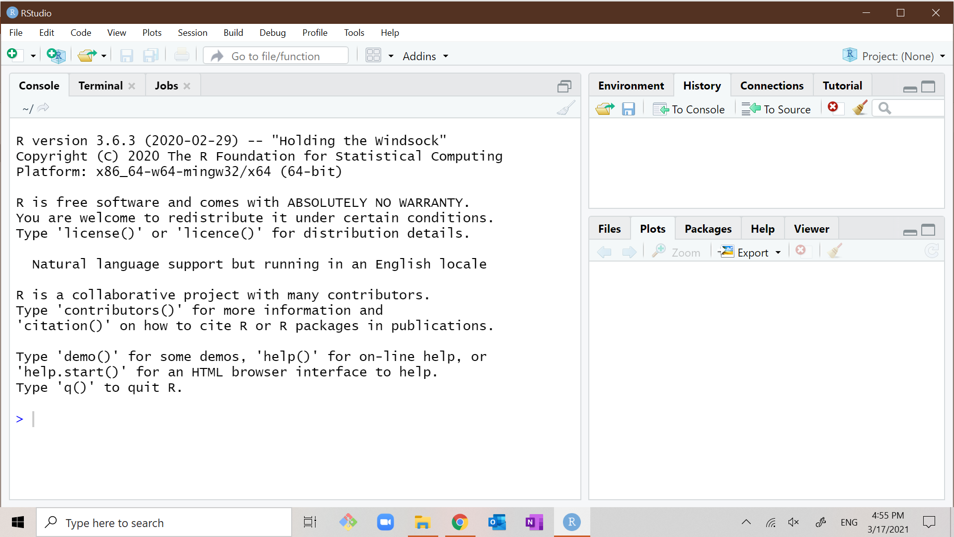
Start the program RStudio. You should see something that looks like
this:
You may wonder what the difference is between R and RStudio.
- R is a programming language designed for statistical analysis.
- R is also the computer program that runs R commands.
- It can also run R scripts, which are just a series of R commands written in a text file.
- RStudio is an integrated development environment (IDE) for
R. It combines R with a set of additional useful tools:
- an interactive session of R (running in the “Console” window).
- a text editor for writing R scripts and R Markdown documents.
- tools for managing files and packages used by R
- tools for comparing and combining scripts and other files
- help and documentation
- many other features
You can run commands and scripts in R itself, but without RStudio you won’t have all these handy extra features. So most people these days use RStudio or another IDE.
RStudio normally displays three or four open windows, each of which has tabs you can select to access different features. We will not use most of them, but some of them will be very handy indeed.
9.1.1 The console window
Like most programming languages, R is designed to execute a series of commands provided by the user. The simplest way to have R execute a command is by entering it into the Console window in the lower left corner.
Example 9.1 Using the console window
Move your cursor into the console window, type the command
print("Hello world!") and press the Enter key to execute the command.
print("Hello world!")
## [1] "Hello world!"
As you type your command in, you may notice that RStudio showed various pop-ups with helpful information about the command. It will also auto-complete your command for you.
R maintains a command history that remembers commands you have previously entered. This is useful when you did something a while ago, but either don’t remember exactly how you did it, or don’t want to type it all in from the beginning.
The simplest way of accessing recent commands is to press the up-arrow key while in the console window.
Example 9.2 Accessing the command history
Suppose you decide you want to say “Hello [your name]!” instead of “Hello world,” and you don’t want to type in the whole command. Then you can:
- Press the up-arrow key in the Console window to show the most recently executed command. If you press it a second time it gives you the command before that, and so on.
- Look at the to the History window in the upper right corner to see a full list of recently executed commands. You can double-click on any command in the window to copy it to the Console window.
Once you have copied the previous command, you can edit it before
pressing <enter>.
9.1.2 Scripts
The Console window is ideal for simple tasks and experimentation, and we will continue using it regularly. But in order to create reproducible research and take full advantage of R’s capabilities, we will need to write and execute scripts.
An script is just a text file containing a sequence of R commands. By
convention, an R script should have the .R extension but any text file will
work.
Example 9.3 Creating an R script
To create an R script
- Select
File > New File > R Scriptfrom the menu. - Enter a valid command in the first line of the file, for example
print("Hello world!") - Enter another valid command in the second line of the file,
for example
print("Goodbye world?") - Select
File > Saveto save your file.- Name it Chapter10Example.R
To run your script:
- Press the
 button.
You will see the results of your commands in the Console window.
9.1.3 R Markdown
RStudio can also run text files written in the R Markdown format. R
Markdown files have the .Rmd extension.
R Markdown is a language for producing documents - HTML files (web pages), Microsoft Word documents, PDF files, etc. - that have R code and analysis embedded in them. In fact, this book is written in R Markdown.
R Markdown is an implementation of the Markdown markup language in R.
What is Markdown?
Markdown is a markup language just like HTML, which means that it is a way of writing documents in text files whose content is readable directly but can also be formatted and displayed (rendered) in a visually appealing way.
The original idea of HTML was that content creators could write their content in text files (pages), with a few HTML tags sprinkled around to give the browser information about structure, and then the browser would display the page. However, as web users demanded fancy graphics, custom colors, interactivity, and mobile-friendly display, HTML became much more complicated.
Markdown was created as radically simplified markup language. The basic idea is to use common conventions for how to indicate structure in a text file.
- Adjacent lines of text are interpreted as part of the same paragraph.
- A line of text following a blank line starts a new paragraph.
- A line of text that begins with “#” is a header, with “#” for level one headers, “##” for level two, etc.
- A line of text that begins with “-” is a bullet point.
- A line of text that begins with a number is part of a numbered list.
- Text written like
*this*is rendered like this. - Text written like
**this**is rendered like this. - Text written like
***this***is rendered like this.
Markdown documents can also include links and pictures (by simply providing the URL or file name), tables, and all sorts of other things.
In addition to ordinary text and Markdown information, R Markdown documents can include pieces of executable R code. R code needs to be surrounded by a code fence that identifies the text inside the fence as R code, and in some cases provides additional information about how it should be executed. This sounds complicated, but is easy to see in a real R Markdown file.
Example 9.4 Creating an R Markdown file
To create our first R Markdown file:
- Select
File > New File > R Markdownfrom the menu.- You will see a dialog box that looks like this:
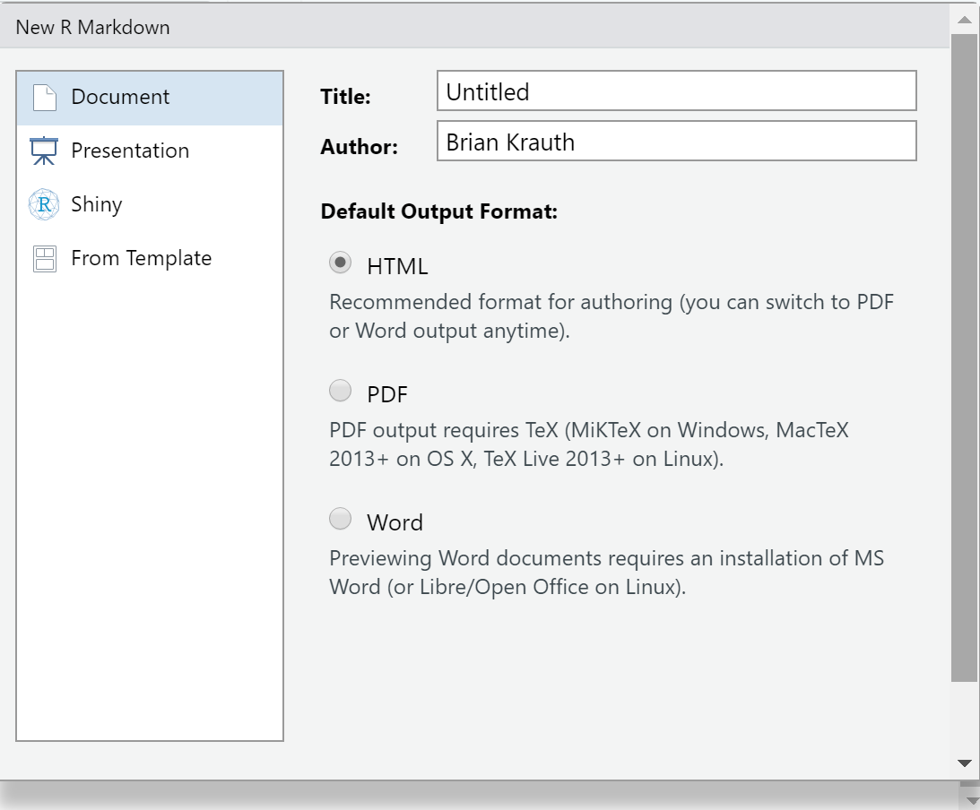
- You will see a dialog box that looks like this:
- The default options are fine, so select
OK. - Save the file.
RStudio has taken the liberty of creating an example R Markdown file that you can use as a template.
You can run the R code in an R Markdown document in one of two ways:
You can run and display results for individual chunks of code. A chunk is a few lines of R code surrounded by a code fence.
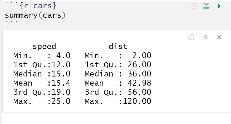
Example 9.5 Running code chunks
To run a code chunk in our R Markdown file:
- Go to the code chunk that looks like this:
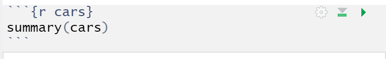
- Press the
 button.
As you can see, the code in the chunk will run and the results
will be displayed below.
You can also knit the entire R Markdown file into an HTML/word/PDF document that includes both the text and the R results by pressing the Knit button.
Example 9.6 Knitting an R Markdown document
To knit an entire document:
- Press the
 button.
It will take a few moments to process the file, and then the HTML file will open in a browser.
By default, R Markdown files usually knit to HTML, but we can knit to other file formats including Word and PDF. We will stick to HTML in this course.
R Markdown resources
R Markdown is as simple or as complicated as you want to make it. A plain text file with a few lines of content is a valid R Markdown file, and like HTML, Markdown is designed so it still “works” if you do something unexpected.
If you want to try something new in R Markdown, or have forgotten how to do something, the most useful resource is the one-page R Markdown Cheat sheet. It is available directly in RStudio, or at https://github.com/rstudio/cheatsheets/raw/master/rmarkdown-2.0.pdf. You can also just search for “r markdown cheatsheet.”
9.1.4 Other RStudio features
RStudio has many other features, most of which we will not use. But I would like to highlight a few that may seem useful.
In the lower right window:
- The Files tab gives you easy access to files in the current active folder.
- The Plots tab will display plots, when you create them.
- The Packages tab is useful for managing packages (more on them later)
- The Help tab allows you to access R’s help system.
In the upper right window
- The Environment tab allows you to view all currently-defined variables and their values.
- The History tab shows the command history.
In the menu:
- You can select
Session > Restart Rto clear the memory and restart the current R session.
We are done for now, so close RStudio. You may get a warning message that
looks something like this:
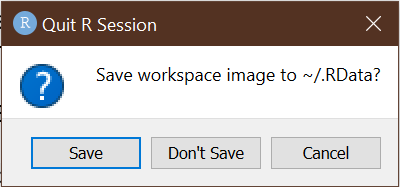
Never click on the Save button here, as it would cause R to
save the current state of its memory and re-load it next time you start R.
In the interest of reproducibility, you should start R “clean” every time.
Click on the Don't Save button, and you will exit RStudio.
9.2 The R language
Next, we will learn some basic features of the R language. Open RStudio and go to the console window so we can enter commands and see what they do.
9.2.1 Expressions
An expression is any piece of R code that can be evaluated on its own. For example:
- Any text, numerical or logical constant:
"Hello world",105,1.34, orTRUE. - Any complete formula built from functions and arithmetic
operators:
log(10)or2+2
An expression needs to be complete, for example ln( is not an
expression, nor is 2+.
Every valid R expression returns a value, also called an object.
- An object can be a number, a text string, a date, or a logical value, just like in Excel.
- Objects can also be much more complex
You can execute any valid R expression as a command, and have it display the value it returns.
# This is a comment. R ignores everything in a line after the '#'
4 + 5
## [1] 9
You can also use any valid R expression within a larger expression.
sqrt(4 + 5)
## [1] 3
In addition, some expressions have a side effect. That is, they make something happen: they cause something to appear on your computer screen, or change a file, or change something in R’s memory.
# This expression has a side effect It causes R to plot a histogram of 100
# N(0,1) random numbers
hist(rnorm(100))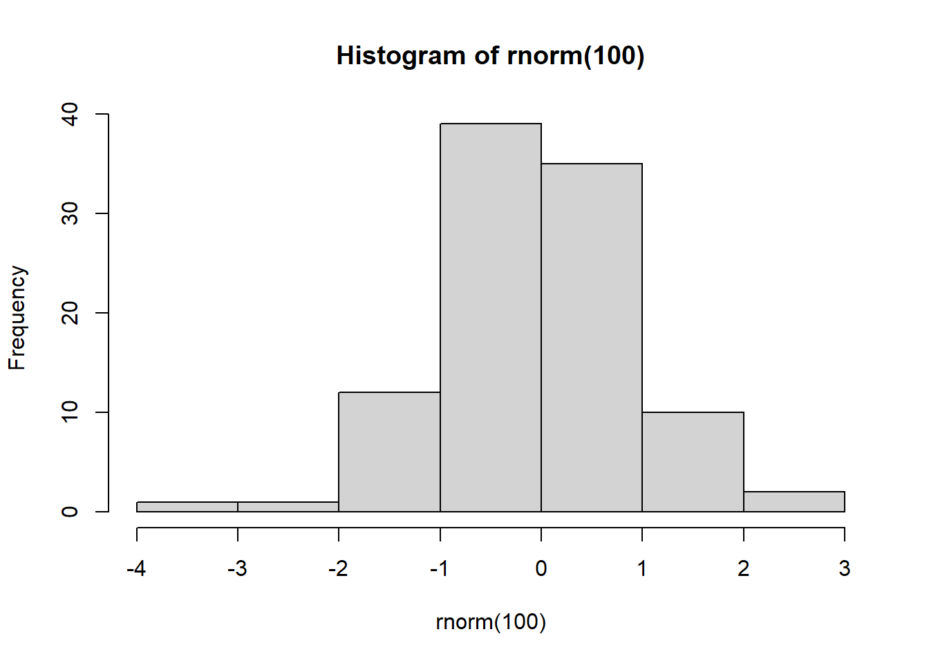
Although we call it a “side effect,” the side effect is often the main purpose of the expression.
9.2.2 Assignment
We can use the <- or assignment operator to assign the results
of an expression to a named variable. We can then use that
variable in later expressions.
For example, the R command x <- 2 assigns the value 2
(i.e., the number 4) to the variable x. Any subsequent code
can then refer to the variable x in its own calculations or
actions.
Example 9.7 Using the assignment operator
# This will cause the variable x to take on the value 2
x <- 2
# We can then use x in any expression
y <- x + 1
print(y)
## [1] 3
# We can change the value of x at any time
x <- 0
# But this will not change the result of any previous calculations
print(y)
## [1] 3
We can display the contents of an object using the print()
function, or by simply giving its name:
x <- 5
print(x)
## [1] 5
x
## [1] 5
9.2.3 Vectors
The primary data structure in R is a vector, which is just an ordered list of elements.
The simplest type of vector is called an atomic vector - its elements are normally from one of R’s basic or atomic data types:
- text strings
- numbers
- logical values (either
TRUEorFALSE)
The elements of an atomic vector need to be all part of the same atomic type; a single vector cannot contain both strings and numbers, for example.
We can construct a vector by enumeration using the c() function:
fruits <- c("Avocado", "Banana", "Cantaloupe")
print(fruits)
## [1] "Avocado"    "Banana"     "Cantaloupe"
There are many other functions that can be used to construct vectors. Two
particularly useful ones are rep which repeats something a particular
number of times, and seq which creates a sequence:
# REP repeats something (like Excel's Fill tool)
ones <- rep(1, times = 10)
print(ones)
##  [1] 1 1 1 1 1 1 1 1 1 1
# SEQ creates a sequence (like Excel's Series tool)
evens <- seq(from = 2, to = 20, by = 2)
print(evens)
##  [1]  2  4  6  8 10 12 14 16 18 20
# You can also create a sequence with the : operator:
print(1:10)
##  [1]  1  2  3  4  5  6  7  8  9 10
Mathematical functions in R operate directly on vectors, and automatically expand scalars (single numbers) to vectors as needed:
# This command subtracts 1 from every element in evens
odds <- evens - ones
print(odds)
##  [1]  1  3  5  7  9 11 13 15 17 19
# This command does the same
odds <- evens - 1
print(odds)
##  [1]  1  3  5  7  9 11 13 15 17 19
The subscript operator [] can be used to select part of a
vector. You can enumerate the indexes of the elements you want:
# You can give a single index evens[2] is the 2nd element in evens
x <- evens[2]
print(x)
## [1] 4
# You can give a vector of indices evens[c(2,5)] is a vector containing the 2nd
# and 5th element in evens
x <- evens[c(2, 5)]
print(x)
## [1]  4 10
# You can give a range of indices evens[2:5] is a vector containing the 2nd,
# 3rd, 4th and 5th element in evens
x <- evens[2:5]
print(x)
## [1]  4  6  8 10
You can also provide logical values instead of numeric indices. R will then
operate on those elements whose corresponding item has the value TRUE:
print(evens)
##  [1]  2  4  6  8 10 12 14 16 18 20
# This creates a vector of the same length as evens, that contains TRUE for all
# values less than 10, and FALSE for all other values
lessthan10 <- (evens < 10)
print(lessthan10)
##  [1]  TRUE  TRUE  TRUE  TRUE FALSE FALSE FALSE FALSE FALSE FALSE
# This creates a vector that includes only those elements of evens for which
# forexample is TRUE
x <- evens[lessthan10]
print(x)
## [1] 2 4 6 8
# This is a quicker way of accomplishing the same result
x <- evens[evens < 10]
print(x)
## [1] 2 4 6 8
Vector subscripting can be used on either side of the assignment operator:
x <- evens
print(x)
##  [1]  2  4  6  8 10 12 14 16 18 20
# This assigns the number 1000 to the 2nd element in x
x[2] <- 1000
print(x)
##  [1]    2 1000    6    8   10   12   14   16   18   20
9.2.4 Lists
The other type of vector is a list. A list is a vector whose elements are themselves other vectors. These vectors can be any type, so we can use lists inside lists to build very complex objects.
Lists can be built using the list() function:
everything <- list(fruits, evens, odds)
print(everything)
## [[1]]
## [1] "Avocado"    "Banana"     "Cantaloupe"
##
## [[2]]
##  [1]  2  4  6  8 10 12 14 16 18 20
##
## [[3]]
##  [1]  1  3  5  7  9 11 13 15 17 19
You can (and should) assign names to the elements of a list:
everything <- list(fruits = fruits, evens = evens, odds = odds)
print(everything)
## $fruits
## [1] "Avocado"    "Banana"     "Cantaloupe"
##
## $evens
##  [1]  2  4  6  8 10 12 14 16 18 20
##
## $odds
##  [1]  1  3  5  7  9 11 13 15 17 19
You can access part of a list by specifying its numerical index inside of the
[[]] operator:
print(everything[[2]])
##  [1]  2  4  6  8 10 12 14 16 18 20
If the items in a list are named, you can also access
them by name using either [[]] or $ notation
print(everything[["evens"]])
##  [1]  2  4  6  8 10 12 14 16 18 20
print(everything$fruits)
## [1] "Avocado"    "Banana"     "Cantaloupe"
You can also use the $ notation to add new items to an existing list:
# There is no element in everything called 'allnumbers'
everything$allnumbers <- c(evens, odds)
# But now there is...
print(everything)
## $fruits
## [1] "Avocado"    "Banana"     "Cantaloupe"
##
## $evens
##  [1]  2  4  6  8 10 12 14 16 18 20
##
## $odds
##  [1]  1  3  5  7  9 11 13 15 17 19
##
## $allnumbers
##  [1]  2  4  6  8 10 12 14 16 18 20  1  3  5  7  9 11 13 15 17 19
9.2.5 Attributes
Any object can also have attributes. This attributes of an object are a list associated with the object that provides additional information.
Let’s see if any of the objects we have created have attributes:
print(attributes(fruits))
## NULL
print(attributes(evens))
## NULL
print(attributes(everything))
## $names
## [1] "fruits"     "evens"      "odds"       "allnumbers"
Note that:
- our two atomic vectors have attributes NULL. That’s R’s way of saying they have no attributes
- our list stores the names of its three elements in
the
$namesattribute.
R has hundreds of standard object types that are built from atomic vectors, lists, and attributes. These object types include matrices, arrays, data sets, objects structured as the output of a particular statistical analysis, descriptions of graphs, and so on. Users can also define their own object types, and there is an extensive system for generic functions and object-based programming (if you know what that is).
9.2.6 Functions and operators
There are hundreds of built-in mathematical and statistical functions in R, and users can easily define their own functions. As you have seen, their format and usage is quite similar to Excel though there are a few important differences.
Let’s get to know the main features of functions in R by considering the
seq() function. We have already seen this function: it is used to
create a vector with a sequence of numbers, much like Excel’s Series
tool.
Every function has a name.
- In our example, the function’s name is
seq.
- In our example, the function’s name is
You can obtain help on any function by entering
?and its name in the console window- Try
? seq.
- Try
Most functions accept one or more arguments.
- The
seqfunction’s arguments includefrom,to,byandlength.out - Every argument has a name and a position. For example,
the
fromargument is in position one, thetoargument is in position two, etc. - Arguments can be passed to the function by name or by position.
- Passing by name looks like this:
seq(from=1,to=5) - Passing by position looks like this:
seq(1,5) - You can mix both methods:
seq(1,5,length.out=10) - I recommend passing by position for simple functions, and passing by name for more complex functions, but it is really just a matter of what works for you.
- Passing by name looks like this:
- Some arguments are required. They must be provided every time the function is called, or else the function will return an error.
- Some arguments are optional. They can be provided, but have
a default value if not provided.
- All arguments to
seq()are optional; execute the commandseq()to see what happens.
- All arguments to
- The
Every function returns a value. This is even true for functions like
print(). To see this:y <- print("Hello world") ## [1] "Hello world" print(y) ## [1] "Hello world"As you can see,
print("Hello world")returns “Hello world” as its value.Some functions also produce side effects, as we have described earlier.
In addition to functions, R has the usual binary mathematical
operators such as +, -, * and /. Operators are
just another way of expressing functions. For example
the + operator is really just another way of calling
the sum() function:
# These two statements are equivalent
2 + 2
## [1] 4
sum(2, 2)
## [1] 4
There are several other commonly used operators:
# Basic arithmetic operators
2 + 3
## [1] 5
2 - 3
## [1] -1
2 * 3
## [1] 6
2/3
## [1] 0.6666667
2^3
## [1] 8
# Comparison operators
2 < 3
## [1] TRUE
2 == 3
## [1] FALSE
2 > 3
## [1] FALSE
# Logical operators
2 == 3 & 2 < 3  # this is logical AND
## [1] FALSE
2 == 3 | 2 < 3  # this is logical OR
## [1] TRUE
The assignment operator is also an operator. It is equivalent to the
assign() function:
# These two statements are equivalent:
x <- 2
assign(y, 2)
print(x)
## [1] 2
print(y)
## [1] "Hello world"
# The assign function returns its own value, so you can do this:
x <- y <- 3
print(x)
## [1] 3
print(y)
## [1] 3
9.3 Packages and the Tidyverse
R has many useful built-in functions and features. But one of its
most useful features is how easy it can be extended by users, and the
fact that it has a large user community who have
provided packages of useful new functions and data.
There are thousands of packages available online. We will use a particularly
useful package called the Tidyverse.
What is the Tidyverse?
The Tidyverse was created by the data scientist Hadley Wickham (also one of the key people behind RStudio) as a way of solving some long-standing problems with R. The Tidyverse is both an R package containing a set of new functions and data structures as well as a philosophy about how to analyze data.
The basic structure of R dates back to 1976 (R itself was created in the early 1990s but is closely based on an earlier program called S). Computer science has advanced a lot since 1976, so some design aspects of R seemed like a good idea at the time but would be designed differently today.
- Too many different ways of doing the same thing
- Too many rarely-used functions,
- Some functions that don’t do what they should.
Unfortunately, we can’t change any of the original functions without causing thousands of existing programs to stop working.
The Tidyverse addresses this problem by replacing many Base R functions with alternative versions that are easier to use, better-designed, and usually faster. It does this in part by being “opinionated” - for example, most data analysis tools in the Tidyverse expect data to be in a tidy format. This reflects a philosophy that data cleaning should precede and be separate from data analysis.
Most commonly-used packages including the Tidyverse are open-source, and are available online from the Comprehensive R Archive Network (CRAN).
Before you can use any package, two steps must be followed:
- The package needs to be installed on your computer using
the
install.packages()function.- This only needs to be done once for each package.
- The package needs to be loaded into memory using the
library()function.- This needs to be done in every R session.
Once the package is installed and loaded, you can use its functions and other features.
Example 9.8 Loading the Tidyverse
You can get a list of all available CRAN packages by simply executing
the install.packages() function with no arguments:
install.packages()If you know the name of the CRAN package you want to install, you can provide it as the argument:
install.packages("tidyverse")You only need to install each package once.
However, installing a package only puts the files on your computer. In order
to actually use the features of a package you need to load it into
memory during your current R session using the library() function:
library("tidyverse")You can then use the Tidyverse functions and other tools.
9.4 Some examples
I have explained some of the basic structure of R, but the best way to learn a tool is by using it.
Example 9.9 Plotting a PDF
Suppose we want to plot the \(N(0,1)\) PDF. We can start by describing step-by-step what we need to do:
- Construct a vector \(x\) of values at which to plot the PDF.
- Calculate a vector \(p = \phi(x)\), where \(\phi(\cdot)\) is the \(N(0,1)\) PDF.
- Plot \(p\) against \(x\).
Then we need to figure out how to accomplish each step using R:
Our first step can be accomplished using the
seq()function, which we have already used. If you know the name of the function you want to use, you can access its help page by executing the command? [function name here]:# ? seqAs you can see, the
seq()function takes argumentsfrom=(for the starting point),to=(for the end point), andlength.out=(for the total number of points). Let’s plot the function at 10 points between -4 and 4:x <- seq(from = -4, to = 4, length.out = 10) print(x) ## [1] -4.0000000 -3.1111111 -2.2222222 -1.3333333 -0.4444444 0.4444444 ## [7] 1.3333333 2.2222222 3.1111111 4.0000000Note that I’ve picked only 10 points here so that our code is easy to check.
The next step is to calculate the standard normal PDF at each of these points. R is a program for statisticians, so it presumably has that PDF available as a built-in function. But what if we don’t know its name? We can just Google “normal pdf in r” and click on a page or two to find out that the function we need is called
dnorm().p <- dnorm(x) print(p) ## [1] 0.0001338302 0.0031560163 0.0337736510 0.1640100747 0.3614238299 ## [6] 0.3614238299 0.1640100747 0.0337736510 0.0031560163 0.0001338302Our last step is to plot \(p\) against \(x\). We could Google, or we could guess that the function for creating plots is called
plot()and try something out. Don’t be scared to try things out, nothing bad could possibly happen here.plot(x, p)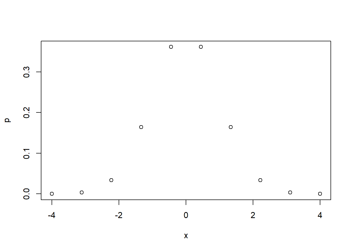 You will see this plot in the Plots tab in the lower right corner
of your screen.
You will see this plot in the Plots tab in the lower right corner
of your screen.
Well, that’s not too bad, but we might want to make some improvements:
- Plot it at more points (1000 rather than 10, for example)
- Connect the points with a line
- Add a title
So we can read through the documentation for the plot() function,
try a few things out, and we can produce a much prettier graph
by just adding a few options:
x <- seq(from = -4, to = 4, length.out = 1000)
p <- dnorm(x)
plot(x, p, type = "l", ylab = expression(phi(x)), main = "PDF of N(0,1) distribution")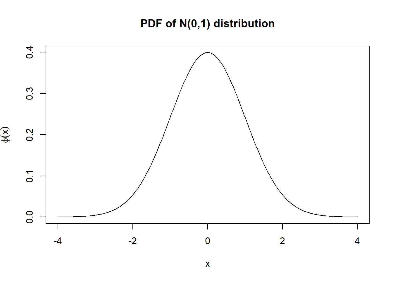
As you can see, we have a much nicer and clearer looking plot.
Chapter review
In this chapter, we learned how to run R programs whether in the console, in a script, or in an R Markdown document. We also learned some basics of the R language. We haven’t learned how to do much of anything useful yet with data, but we will over the next few chapters. In particular, we will learn how to move data from Excel to R, how to view data in R, and how to clean and analyze data in R. We will also learn a sophisticated R graphing package called ggplot.
Although you will be tested on specific knowledge, you should also keep in mind the bigger picture: my real goal here is for you to develop some long-lasting skills that you will find useful in the future. This should be your goal as well.
A year from now, or five years from now, you will probably not be able
to remember exactly what the format of the seq function is, nor will
you need to. Instead I want you to focus on learning how to think about
a coding task, how to find information, and how to design and implement
your plans.
For more information on R
There are many free sources of useful information about R.
- A good short introduction is available at https://cran.r-project.org/doc/contrib/Torfs+Brauer-Short-R-Intro.pdf.
- A good longer book that focuses on the Tidyverse is Wickham and Grolemund’s R for Data Science. It can be purchased as an actual book from Amazon or your local book shop, and is also available as a free e-book at https://r4ds.had.co.nz/index.html.
Practice problems
Answers can be found in the appendix.
SKILL #1: Perform basic tasks in RStudio
- Open RStudio and do the following:
- Execute a command in the console window.
- Write and execute (source) a brief script.
- Write and knit a brief R Markdown document.
SKILL #2: Use R expressions and vectors
- Which of the following are valid R expressions?
"Hello world"HelloHello"2+2x <- 2 + 2x <- 2 +
- Write the R code to perform the following actions:
- Create a vector named
cookiesthat contains the elements “oatmeal,” “chocolate chip,” and “shortbread.” - Create a vector named `
threesthat contains all of the integers between 1 and 100 that are divisible by 3. - Use the vector
threesto find the 5th-lowest integer between 1 and 100 that is divisible by 3. - Create a list named
threecookiesthat containscookiesandthrees.
- Create a vector named
SKILL #3: Use R packages
Load the tidyverse package (you will need to install it if you have not already done so), and execute the R code below:
data("mtcars")  # load data
ggplot(mtcars, aes(wt, mpg)) + geom_point(aes(colour=factor(cyl), size = qsec))