Chapter 4 Introduction to random variables

The previous chapter developed a general framework for modeling random outcomes and events. This framework can be applied to any set of random outcomes, no matter how complex.

This chapter develops additional tools for the case when the random outcomes we are interested in are quantitative, that is, they can be described by a number. Quantitative outcomes are also called “random variables.”

Chapter goals

In this chapter we will learn how to:

Calculate and interpret the CDF and PDF of a discrete random variable, or several random variables.
Calculate and interpret the expected value of a discrete random variable from its PDF.
Calculate and interpret the variance and standard deviation of a discrete random variable from its PDF.
Work with common discrete probability distributions including the Bernoulli, binomial, and discrete uniform.

The material in this chapter will use some mathematical notation (the summation operator) that provides a convenient way to represent long sums. Please review the section on sequences and summations in the math appendix.

4.1 Random variables

A random variable is a number whose value depends on a random outcome. The idea here is that we are going to use a random variable to describe some (but not necessarily every) aspect of the outcome.

Example 4.1 Random variables in roulette

Here are a few random variables we could define in a roulette game:

The original outcome $b$.
An indicator for whether a bet on red wins: \[r = I(b \in Red)=\begin{cases}1 & b \in Red\\ 0 & b \notin Red \\ \end{cases}\]
The net payout from a $1 bet on red: \[ w_{red} = w_{red}(b) = \begin{cases} 1 & \textrm{ if } b \in Red \\ -1 & \textrm{ if } b \in Red^c \end{cases} \] That is, a player who bets $1 on red wins $1 if the ball lands on red and loses $1 if the ball lands anywhere else.
The net payout from a $1 bet on 14: \[ w_{14} = w_{14}(b) = \begin{cases} 35 & \textrm{ if } b = 14 \\ -1 & \textrm{ if } b \neq 14 \end{cases} \] That is, a player who bets $1 on 14 wins $35 if the ball lands on 14 and loses $1 if the ball lands anywhere else.

All of these random variables are defined in terms of the underlying outcome.

A random variable is always a function of the original outcome, but for convenience, we usually leave its dependence on the original outcome implicit, and write it as if it were an ordinary variable.

4.1.1 Implied distribution

A random variable has its own sample space (normally $\mathbb{R}$) and probability distribution. This probability distribution can be derived from the probability distribution of the underlying outcome.

Example 4.2 Probability distributions for roulette

The probability distribution for $b$ is: \[\Pr(b = 0) = 1/37 \approx 0.027\] \[\Pr(b = 1) = 1/37 \approx 0.027\] \[\vdots\] \[\Pr(b = 36) = 1/37 \approx 0.027\] All other values of $b$ have probability zero.
The probability distribution for $w_{red}$ is: \[\Pr(w_{red} = 1) = \Pr(b \in Red) = 18/37 \approx 0.486\] \[\Pr(w_{red} = -1) = \Pr(b \notin Red) = 19/37 \approx 0.514\] All other values of $w_{red}$ have probability zero.
The probability distribution for $w_{14}$ is: \[\Pr(w_{14} = 35) = \Pr(b = 14) = 1/37 \approx 0.027\] \[\Pr(w_{14} = -1) = \Pr(b \neq 14) = 36/37 \approx 0.973\] All other values of $w_{14}$ have probability zero.

Notice that these random variables are related to each other since they all depend on the same underlying outcome. Section 5.4 will explain how we can describe and analyze those relationships.

4.1.2 The support

The support of a random variable $x$ is the smallest³ set $S_x \subset \mathbb{R}$ such that $\Pr(x \in S_x) = 1$.

In plain language, the support is the set of all values in the sample space that have some chance of actually happening.

Example 4.3 The support in roulette

The support of $b$ is $S_{b} = \{0,1,2,\ldots,36\}$.

The support of $w_{Red}$ is $S_{Red} = \{-1,1\}$.

The support of $w_{14}$ is $S_{14} = \{-1,35\}$.

The random variables we will consider in this chapter have discrete support. That is, the support is a set of isolated points each of which has a strictly positive probability. In most examples the support will also have a finite number of elements. All finite sets are also discrete, but it is also possible for a discrete set to have an infinite number of elements. For example, the set of integers is both discrete and infinite.

Some random variables have a support that is continuous rather than discrete. Chapter 5 will cover continuous random variables.

4.1.3 The PDF

We can describe the probability distribution of a random variable with a function called its probability density function (PDF).

The PDF of a discrete random variable is defined as: \[f_x(a) = \Pr(x = a)\] where $a$ is any number. By convention, we typically use a lower-case $f$ to represent a PDF, and we use the subscript when needed to clarify which specific random variable we are talking about.

Example 4.4 The PDF in roulette

Our three random variables are all discrete, and each has its own PDF:

\[f_b(a) = \Pr(b = a) = \begin{cases} 1/37 & a \in \{0,1,\ldots,36\} \\ 0 & a \notin \{0,1,\ldots,36\} \\ \end{cases}\] \[f_{red}(a) = \Pr(w_{red} = a) = \begin{cases} 19/37 & a = -1 \\ 18/37 & a = 1 \\ 0 & a \notin \{-1,1\} \\ \end{cases}\] \[f_{14}(a) = \Pr(w_{14} = a) = \begin{cases} 36/37 & a = -1 \\ 1/37 & a = 35 \\ 0 & a \notin \{-1,35\} \\ \end{cases}\]

Figure 4.1 below shows these three PDFs.

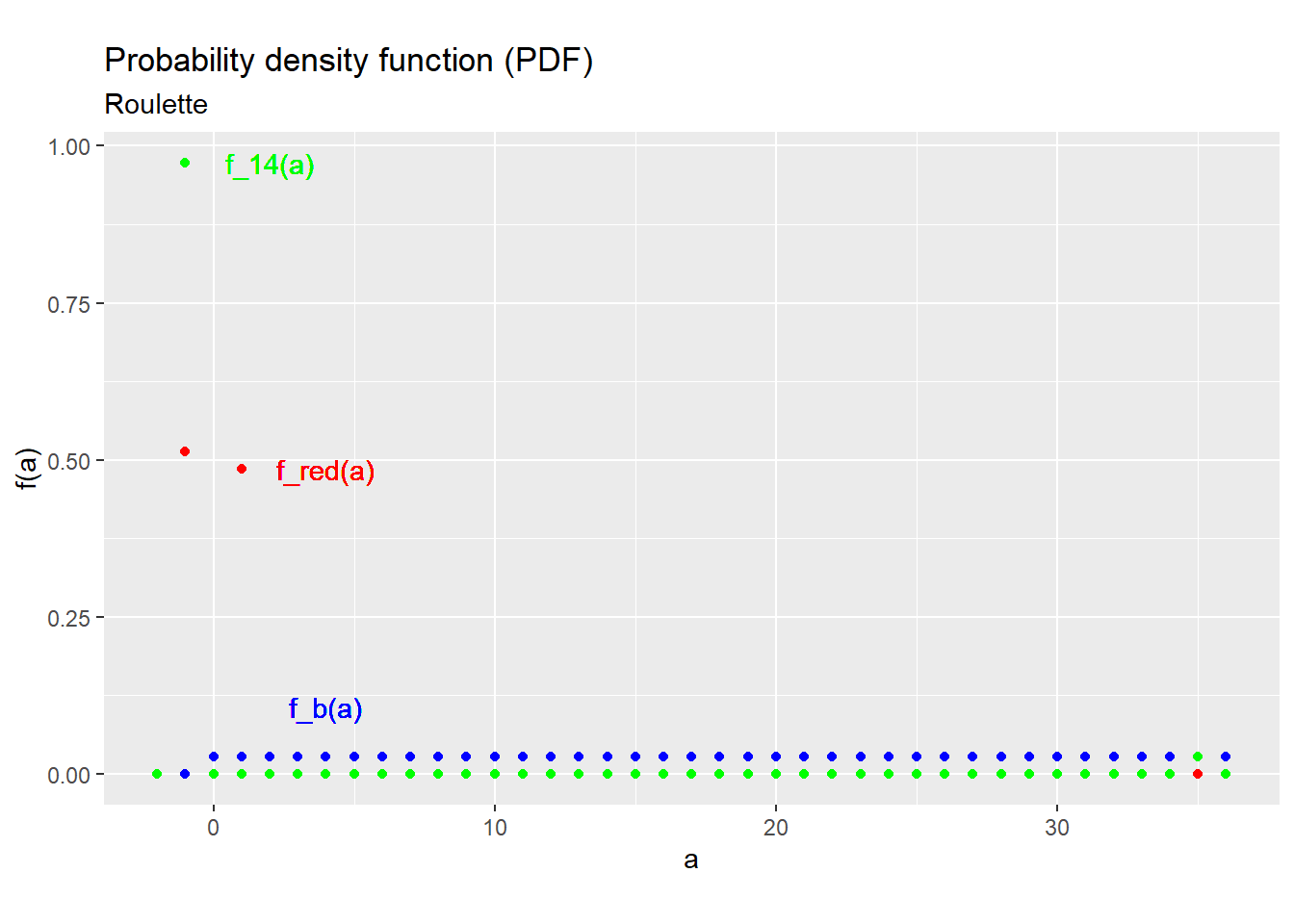
Figure 4.1: PDFs for the roulette example

We can calculate any probability from the PDF by simple addition. That is: \[\Pr(x \in A) = \sum_{s \in S_x} f_x(s)I(s \in A)\] where⁴ $A \subset \mathbb{R}$ is any event defined for $x$.

Example 4.5 Some event probabilities in roulette

Since the outcome in roulette is discrete, we can calculate any event probability by adding up the probabilities of the event’s outcomes.

The probability of the event $b \leq 3$ can be calculated: \[\begin{align} \Pr(b \leq 3) &= \sum_{s=0}^{36}f_x(s)I(s \leq 3) \\ &= f_b(0) + f_b(1) + f_b(2) + f_b(3) \\ &= 4/37 \end{align}\]

The probability of the event $b \in Even$ can be calculated: \[\begin{align} \Pr(b \in Even) &= \sum_{s=0}^{36}f_x(s)I(s \in Even) \\ &= f_b(2) + f_b(4) + \cdots + f_b(36) \\ &= 18/37 \end{align}\]

The PDF of a discrete random variable has several general properties:

It is always between zero and one: \[0 \leq f_x(a) \leq 1\] since it is a probability.
It sums up to one over the support: \[\sum_{a \in S_x} f_x(a) = \Pr(x \in S_x) = 1\] since the support has probability one by definition.
It is strictly positive for all values in the support: \[a \in S_x \implies f_x(a) > 0\] since the support is the smallest set that has probability one.

You can confirm that examples above all satisfy these properties.

4.1.4 The CDF

Another way to describe the probability distribution of a random variable is with a function called its cumulative distribution function (CDF). The CDF is a little less intuitive than the PDF, but it has the advantage that it always has the same definition whether or not the random variable is discrete.

The CDF of the random variable $x$ is the function $F_x:\mathbb{R} \rightarrow [0,1]$ defined by: \[F_x(a) = Pr(x \leq a)\] where $a$ is any number. By convention, we typically use an upper-case $F$ to indicate a CDF, and we use the subscript to indicate what random variable we are talking about.

We can construct the CDF of a discrete random variable by just adding up the PDF: \[\begin{align} F_x(a) &= \Pr(x \leq a) \\ &= \sum_{s \in S_x} f_x(s)I(s \leq a) \end{align}\] This formula leads to a “stair-step” appearance: the CDF is flat for all values outside of the support, and then jumps up at all values in the support.

Example 4.6 CDFs for roulette

The CDF of $b$ is: \[F_b(a) = \begin{cases} 0 & a < 0 \\ 1/37 & 0 \leq a < 1 \\ 2/37 & 1 \leq a < 2 \\ \vdots & \vdots \\ 36/37 & 35 \leq a < 36 \\ 1 & a \geq 36 \\ \end{cases}\]
The CDF of $w_{red}$ is: \[F_{red}(a) = \begin{cases} 0 & a < -1 \\ 19/37 & -1 \leq a < 1 \\ 1 & a \geq 1 \\ \end{cases}\]
The CDF of $w_{14}$ is: \[F_{14}(a) = \begin{cases} 0 & a < -1 \\ 36/37 & -1 \leq a < 35 \\ 1 & a \geq 35 \\ \end{cases}\]

The CDF has several properties. First, it is non-decreasing. That is, choose any two numbers $a$ and $b$ so that $a \leq b$. Then \[F_x(a) \leq F_x(b)\] The reason for this is simple: the event $x \leq a$ implies the event $x \leq b$, so its probability cannot be higher.

Second, it is a probability, which implies: \[0 \leq F_x(a) \leq 1\] just like for a discrete PDF.

Third, it runs from zero to one: \[\lim_{a \rightarrow -\infty} F_x(a) = \Pr(x \leq -\infty) = 0\] \[\lim_{a \rightarrow \infty} F_x(a) = \Pr(x \leq \infty) = 1\] The intuition is simple: all values in the support are between $-\infty$ and $\infty$.

Example 4.7 CDF properties

Figure 4.2 below graphs the CDFs from the previous example:

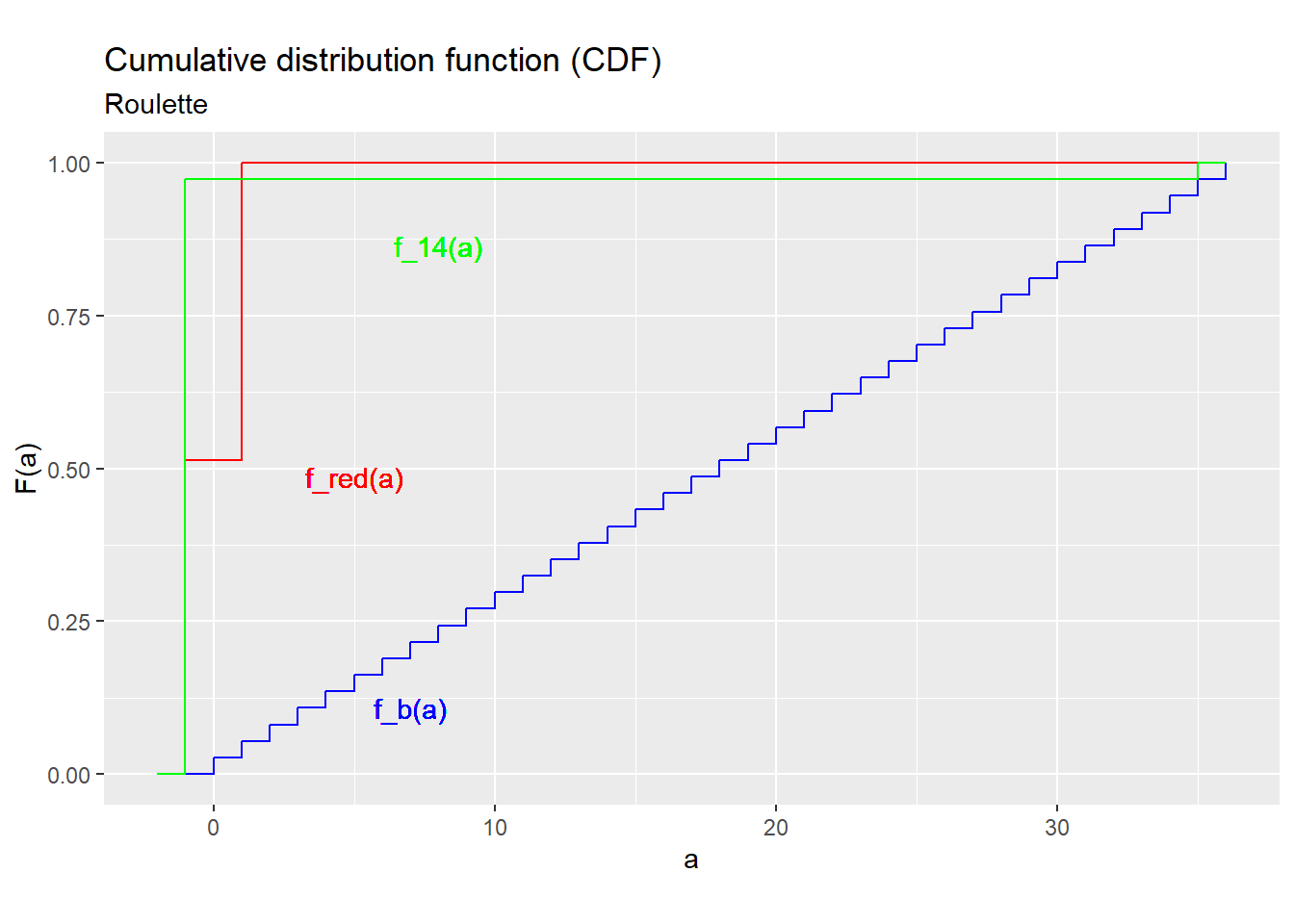
Figure 4.2: CDFs for the roulette example

Notice that they show all of the general properties described above.

The CDF never goes down, only goes up or stays the same.
The CDF runs from zero to one, and never leaves that range.

In addition, all of these CDFs have a distinctive “stair-step” shape, jumping up at each point in $S_x$ and flat between those points, This is a general property of CDFs for discrete random variables.

In addition to constructing the CDF from the PDF, we can also go the other way, and construct the PDF of a discrete random variable from its CDF. Each little jump in the CDF is a point in the support, and the size of the jump is exactly equal to the PDF.

In more formal mathematics, the formula for deriving the PDF of a discrete random variable from its CDF would be written:

\[f_x(a) = \lim_{\epsilon \rightarrow 0} F_x(a) - F_x(a-|\epsilon|)\] but we can just think of it as the size of the jump.

Finally, we can use the CDF to calculate the probability that $x$ lies in any interval. That is, let $a$ and $b$ be any two numbers such that $a < b$. Then: \[\begin{align} F(b) - F(a) &= \Pr(x \leq b) - \Pr(x \leq a) \\ &= \Pr((x \leq a) \cup (a < x \leq b)) - \Pr(x \leq a) \\ &= \Pr(x \leq a) + \Pr(a < x \leq b) - \Pr(x \leq a) \\ &= \Pr(a < x \leq b) \end{align}\] Notice that we have to be a little careful here to distinguish between the strict inequality $<$ and the weak inequality $\leq$, because it is always possible for $x$ to be exactly equal to $a$ or $b$.

Example 4.8 Calculating interval probabilities

Consider the CDF for $b$ derived above. Then: \[\begin{align} \Pr(b \leq 36) &= F_b(36) &=1 \\ \Pr(1 < b \leq 36) = F_b(36) - F_b(1) \\ &= 1 - 2/37 \\ &= 35/37 \end{align}\]

4.1.5 Functions of a random variable

Any function of a random variable is also a random variable. So for example, if $x$ is a random variable, so is $x^2$ or $\ln (x)$ or $\sqrt{x}$. We can derive the PDF or CDF of a function of a random variable directly from the PDF or CDF of the original random variable.

We say that $y$ is a linear function of $x$ if: \[y = ax + b\] where $a$ and $b$ are constants. We will have many results that apply specifically for linear functions.

Example 4.9 A linear function in roulette

The net payout from a $1 bet on red ($w_{red}$) was earlier defined directly from the underlying outcome $b$. However, we could have also defined it as a linear function of the random variable $r$: \[w_{red} = 2r-1\] That is, $w_{red} = -1$ when red loses ($r = 0$) and $w_{red} = 1$ when red wins ($r = 1$).

4.2 The expected value

The expected value of a random variable $x$ is written $E(x)$. When $x$ is discrete, it is defined as:

\[E(x) = \sum_{a \in S_x} a\Pr(x=a) = \sum_{a \in S_x} af_x(a)\] The expected value is also called the mean, the population mean or the expectation of the random variable.

The formula might look difficult if you are not used to the notation, but it is actually quite simple to calculate:

Figure out the set of values in the support of $x$.
Multiply each value in the support by the PDF at that value.
Add these all up.

Example 4.10 Some expected values in roulette

The support of $b$ is $\{0,1,2\ldots,36\}$ so its expected value is: \[\begin{align} E(b) &= 0*\underbrace{f_b(0)}_{1/37} + 1*\underbrace{f_b(1)}_{1/37} + \cdots 36*\underbrace{f_b(36)}_{1/37} \\ &= 18 \end{align}\]

The support of $r$ is $\{0,1\}$ so its expected value is: \[\begin{align} E(r) &= 0*\underbrace{f_r(0)}_{19/37} + 1*\underbrace{f_r(1)}_{18/37} \\ &= 18/37 \\ &\approx 0.486 \end{align}\]

The support of $w_{14}$ is $\{-1,35\}$ so its expected value is: \[\begin{align} E(w_{14}) &= -1*\underbrace{f_{14}(-1)}_{36/37} + 35*\underbrace{f_{14}(35)}_{1/37} \\ &= 1/37 \\ &\approx -0.027 \end{align}\] That is, each dollar bet on 14 leads to an average loss of 2.7 cents for the bettor.

We can think of the expected value as a weighted average of its possible values, with each value weighted by the probability of observing that value.

Since the expected value is a sum, it has some of the same properties as sums. In particular, the associative and distributive rules apply, which means that: \[E(a + bx) = a + bE(x)\] That is, we can take the expected value “inside” any linear function. This will turn out to be a very handy property.

Example 4.11 The expected value of a linear function in roulette

Earlier, we showed that $w_{red}$ is a linear function of $r$: \[w_{red} = 2r -1\] so its expected value is: \[E(w_{red}) = E(2r - 1) = 2 \underbrace{E(r)}_{18/37} - 1 = -1/37 \approx -0.027\] We can verify this calculation is correct by deriving the expected value directly from the PDF: \[E(w_{red}) = -1*\underbrace{f_{red}(-1)}_{19/37} + 1*\underbrace{f_{red}(1)}_{18/37} \approx -0.027\] That is, each dollar bet on red leads to an average loss of 2.7 cents for the bettor, as does each dollar bet on 14.

Unfortunately, this handy property applies only to linear functions. If $g(\cdot)$ is a nonlinear function, than $E(g(x)) \neq g(E(x))$. For example: \[E(x^2) \neq E(x)^2\] \[E( 1/x ) \neq 1 / E(x)\] Students frequently make this mistake, so try to avoid it.

Example 4.12 The expected value of a nonlinear function in roulette

We can define $w_{14}$ as a function of the underlying outcome $b$: \[w_{14} = 36 I(b = 14) -1\] That is, $w_{14}=35$ if a bet on 14 wins ($b = 14$) and $w_{14}= -1$ otherwise. Although this is a linear function of the indicator variable $I(b=14)$, it is a nonlinear function of $b$ itself.

If we could take the expected value inside of a nonlinear function we would get: \[\begin{align} E(w_{14}) &= 36 I(\underbrace{E(b)}_{18}=14) - 1 \qquad \textrm{(can we do this?)} \\ &= 36 \underbrace{I(18=14)}_{0} - 1 \\ &= -1 \end{align}\] which is clearly wrong since we already calculated that $E(w_{14}) = -0.027$.

4.3 Other characteristics

The expected value is one way of describing something about a random variable, but there are many others. We will describe a few of the most important ones.

4.3.1 Range

The range of a random variable is the interval from its lowest possible value ($\min(S_x)$ its highest possible value $\max(S_x)$.

Example 4.13 The range in roulette

The support of $w_{red}$ is $\{-1,1\}$ so its range is $[-1,1]$.

The support of $w_{14}$ is $\{-1,35\}$ so its range is $[-1,35]$.

The support of $b$ is $\{0,1,2,\ldots,36\}$ so its range is $[0,36]$.

4.3.2 Quantiles and percentiles

Let $q$ be any number between zero and one. Then the $q$ quantile of a random variable $x$ is defined as: \[F_x^{-1}(q) = \min\{a: \Pr(x \leq a) \geq q\} = \min\{a: F_x(a) \geq q\}\] where $F_x(\cdot)$ is the CDF of $x$. The quantile function $F_x^{-1}(\cdot)$ is also called the inverse CDF.

The $q$ quantile of a distribution is also called the $100q$ percentile; for example the 0.25 quantile of $x$ is also called the 25th percentile of $x$.

Example 4.14 Quantiles in roulette

The CDF of $w_{red}$ is: \[F_{red}(a) = \begin{cases}0 & a < -1 \\ 0.514 & -1 \leq a < 1 \\ 1 & a \geq 1 \\ \end{cases}\] We can plot this CDF below.

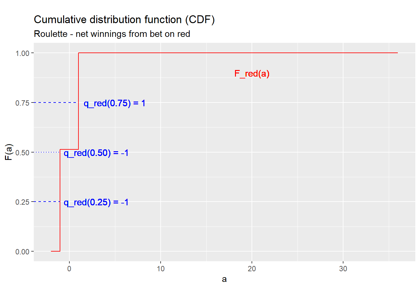
Figure 4.3: CDFs for the roulette example

We can use this graph to find any quantile. For example, the 0.25 quantile (25th percentile) is: \[F_{red}^{-1}(0.25) = \min\{a: \Pr(w_{red} \leq a) \geq 0.25\} = \min [-1,1] = -1\] which is depicted by the lowest blue dashed line.

By the same method, we can find that the 0.5 quantile (50th percentile) is: \[F_{red}^{-1}(0.5) = \min\{a: \Pr(w_{red} \leq a) \geq 0.5\} = \min [-1,1] = -1\] and the 0.75 quantile (75th percentile) is: \[F_{red}^{-1}(0.75) = \min\{a: \Pr(w_{red} \leq a) \geq 0.75\} = \min\{1\} = 1\]

The formula for the quantile function may look intimidating, but it can be constructed by just “flipping” the axes of the CDF.

Example 4.15 The whole quantile function

The quantile function for $w_{red}$ can be constructed by inverting the $F_{red}(\cdot)$:

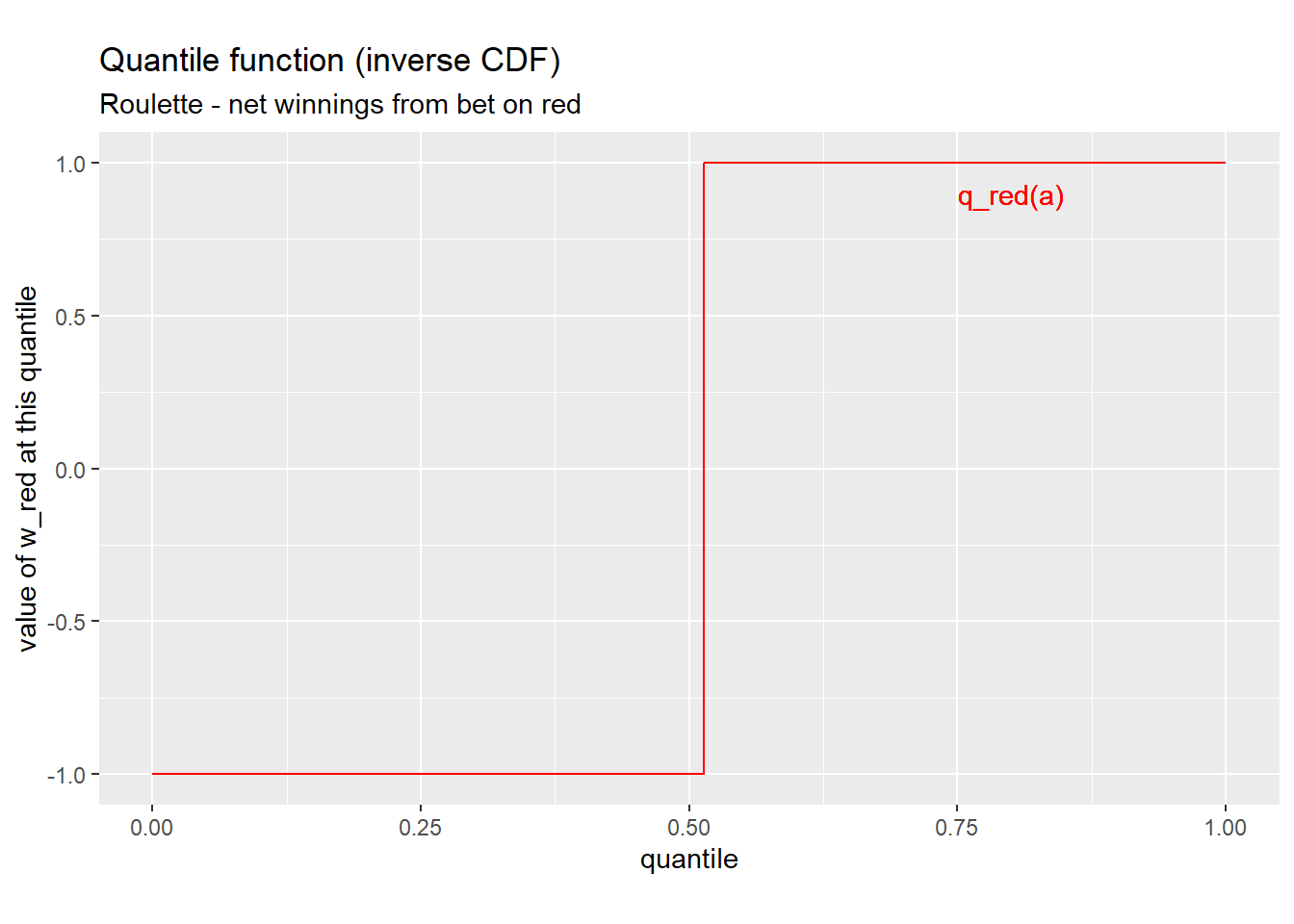
Figure 4.4: Quantile function for w_red

4.3.3 Median

The median of a random variable is its 0.5 quantile or 50th percentile. It can be interpreted roughly as the “middle” of the distribution.

Example 4.16 The median in roulette

The median of $w_{red}$ is just its 0.5 quantile or 50th percentile: \[median(w_{red}) = F_{red}^{-1}(0.5) = -1\]

4.3.4 Variance

The median and expected value both aim to describe a typical or central value of the random variable. We are also interested in measures of how much the random variable varies. We have already seen one - the range - but there are others, including the variance and standard deviation.

The variance of a random variable $x$ is defined as: \[\sigma_x^2 = var(x) = E((x-E(x))^2)\] Variance can be thought of as a measure of how much $x$ tends to deviate from its central tendency $E(x)$.

Example 4.17 Calculating variance from the definition

The variance of $r$ is: \[\begin{align} var(r) &= (0-\underbrace{E(r)}_{18/37})^2 *\frac{19}{37} + (1-\underbrace{E(r)}_{18/37})^2 * \frac{18}{37} \\ &\approx 0.25 \end{align}\] The variance of $w_{red}$ is: \[\begin{align} var(w_{red}) &= (-1-\underbrace{E(w_{red})}_{\approx 0.027})^2 * \frac{19}{37} + (1-\underbrace{E(w_{red})}_{\approx 0.027})^2 * \frac{18}{37} \\ &\approx 1.0 \end{align}\]

The variance of $w_{14}$ is \[\begin{align} var(w_{14}) &= (-1-\underbrace{E(w_{14})}_{\approx 0.027})^2 * \frac{36}{37} + (35-\underbrace{E(w_{14})}_{\approx 0.027})^2 * \frac{1}{37} \\ &\approx 34.1 \end{align}\]

That is, a bet on 14 has the same expected payout as a bet on red, but its payout is much more variable.

The key to understanding the variance is that it is the expected value of a square $(x-E(x))^2$, and the expected value is just a (weighted) sum.

The first implication of this is that the variance is always positive (or more precisely, non-negative): \[var(x) \geq 0\] The intuition is straightforward. All squares are positive, and the expected value is just a sum. If you add up several positive numbers, you will get a positive number.

The second implication is that: \[var(x) = E(x^2) - E(x)^2\] The derivation of this is as follows: \[\begin{align} var(x) &= E((x-E(x))^2) \\ &= E( ( x-E(x) ) * (x - E(x) )) \\ &= E( x^2 - 2xE(x) + E(x)^2) \\ &= E(x^2) - 2E(x)E(x) + E(x)^2 \\ &= E(x^2) - E(x)^2 \end{align}\] This formula is often an easier way of calculating the variance.

Example 4.18 Another way of calculating the variance

We already found that $E(w_{14}) = -0.027$, so we can calculate $var(w_{14})$ by finding: \[\begin{align} E(w_{14}^2) &= (-1)^2 f_{14}(-1) + 35^2 f_{14}(35) \\ &= 1 * \frac{36}{37} + 1225 * \frac{1}{37} \\ &\approx 34.08 \end{align}\] Adding these together we get: \[\begin{align} var(w_{14}) &= E(w_{14}^2) - E(w_{14})^2 \\ &\approx 34.08 + (-0.027)^2 \\ &\approx 34.1 \end{align}\] That is, a bet on 14 has the same expected payout as a bet on red, but its payout is much more variable.

We can also find the variance of any linear function of a random variable. For any constants $a$ and $b$: \[var(a + bx) = b^2 var(x)\] This can be derived as follows: \[\begin{align} var(a+bx) &= E( ( (a+bx) - E(a+bx))^2) \\ &= E( ( a+bx - a-bE(x))^2) \\ &= E( (b(x - E(x)))^2) \\ &= E( b^2(x - E(x))^2) \\ &= b^2 E( (x - E(x))^2) \\ &= b^2 var(x) \end{align}\] I do not expect you to remember how to derive these results, but I want you to know them and use them.

Example 4.19 Variance of a linear function

The variance of $w_{red}$ is: \[\begin{align} var(w_{red}) &= var( 2r - 1) \\ &= 2^2 var(r) \\ &\approx 4*0.25 \\ &\approx 1.0 \end{align}\]

4.3.5 Standard deviation

The standard deviation of a random variable is defined as the (positive) square root of its variance. \[\sigma_x = sd(x) = \sqrt{var(x)}\] The standard deviation is just another way of describing the variability of $x$.

In some sense, the variance and standard deviation are interchangeable since they are so closely related. The standard deviation has the advantage that it is expressed in the same units as the underlying random variable, while the variance is expressed in the square of those units. This makes the standard deviation somewhat easier to interpret.

Example 4.20 Standard deviation in roulette

The standard deviation of $r$ is: \[sd(r) = \sqrt{var(r)} \approx 0.5\]

The standard deviation of $w_{red}$ is: \[sd(w_{red}) = \sqrt{var(w_{red})} \approx 1.0\]

The standard deviation of $w_{14}$ is \[sd(w_{14}) = \sqrt{var(w_{14})} \approx 5.8\]

The standard deviation has analogous properties to the variance:

It is always non-negative: \[sd(x) \geq 0\]
For any constants $a$ and $b$: \[sd(a +bx) = b \, sd(x)\]

These properties follow directly from the corresponding properties of the variance.

4.4 Standard discrete distributions

In principle, there are an infinite number of possible probability distributions. However, some probability distributions appear so often in applications that we have given them names. This provides a quick way to describe a particular distribution without writing out its full PDF, using the notation \[RandomVariable \sim DistributionName(Parameters)\] where $RandomVariable$ is the name of the random variable whose distribution is being described, the $\sim$ character can be read as “has the following probability distribution,” $DistributionName$ is the name of the probability distribution, and $Parameters$ is a list of numbers called parameters that provide additional information about the probability distribution.

Using a standard distribution also allows us to establish the properties of a commonly-used distribution once, and use those results every time we use that distribution.

4.4.1 Bernoulli

The Bernoulli probability distribution is usually written: \[x \sim Bernoulli(p)\] It has discrete support $S_x = \{0,1\}$ and PDF: \[f_x(a) = \begin{cases} (1-p) & a = 0 \\ p & a = 1 \\ 0 & a = \textrm{anything else}\\ \end{cases}\] Note that the “Bernoulli distribution” isn’t really a (single) probability distribution. Instead it is what we call a parametric family of distributions. That is, the $Bernoulli(p)$ is a different distribution with a different PDF for each value of the parameter $p$.

We typically use Bernoulli random variables to model the probability of some random event $A$. If we define $x$ as the indicator variable $x=I(A)$, then $x \sim Bernoulli(p)$ where $p=\Pr(A)$.

Example 4.21 The Bernoulli distribution in roulette

The variable $r = I(Red)$ has the $Bernoulli(18/37)$ distribution.

The mean of a $Bernoulli(p)$ random variable is: \[\begin{align} E(x) &= (1-p)*0 + p*1 \\ &= p \end{align}\] and its variance is: \[\begin{align} var(x) &= E[(x-E(x))^2] \\ &= E[(x-p)^2] \\ &= (1-p)(0-p)^2 + p(1-p)^2 \\ &= p(1-p) \end{align}\]

4.4.2 Binomial

The binomial probability distribution is usually written: \[x \sim Binomial(n,p)\] It has discrete support $S_x = \{0,1,2,\ldots,n\}$ and its PDF is: \[f_x(a) = \begin{cases} \frac{n!}{a!(n-a)!} p^a(1-p)^{n-a} & a \in S_x \\ 0 & \textrm{anything else} \\ \end{cases}\] You do not need to memorize or even understand this formula. The Excel function BINOMDIST() can be used to calculate the PDF or CDF of the binomial distribution, and the function BINOM.INV() can be used to calculate its quantiles.

The binomial distribution is typically used to model frequencies or counts. We can show that it is the distribution of how many times a probability-$p$ event happens in $n$ independent attempts.

For example, the basketball player Stephen Curry makes about 43% of his 3-point shot attempts. If each shot is independent of the others, then the number of shots he makes in 10 attempts will have the $Binomial(10,0.43)$ distribution.

Example 4.22 The binomial distribution in roulette

Suppose we play 50 games of roulette, and bet on red in every game. Let $WIN50$ be the number of times we win.

Since the outcome of a single bet on red is $r \sim Bernoulli(18/37)$, this means that $WIN50 \sim Binomial(50,18/37)$.

The mean and variance of a binomial random variable are: \[E(x) = np\] \[var(x) = np(1-p)\]

The formula for the binomial PDF looks strange, but it can actually be derived from a fairly simple and common situation. Let $(b_1,b_2,\ldots,b_n)$ be a sequence of $n$ independent random variables from the $Bernoulli(p)$ distribution and let: \[x = \sum_{i=1}^n b_i\] count up the number of times that $b_i$ is equal to one (i.e., the event modeled by $b_i$ happened). Then it is possible to derive the PDF for $y$, and that is the PDF we call $Binomial(n,p)$. The derivation is not easy, but the intuition is simple:

We can calculate the probability of the event $x=a$ by adding up probability of its component outcomes.
The number of outcomes in the event $x=a$ is $\frac{n!}{a!(n-a)!}$.
The probability of each individual outcome in the event $x=a$ is $p^a(1-p)^{n-a}$.

Therefore the probability of the event $x=a$ is $\frac{n!}{a!(n-a)!}p^a(1-p)^{n-a}$.

4.4.3 Discrete uniform

The discrete uniform distribution \[x \sim DiscreteUniform(S_x)\] is a distribution that puts equal probability on every value in a discrete set $S_x$. Its support is $S_x$ and its PDF is: \[f_x(a) = \begin{cases} 1/|S_x| & a \in S_x \\ 0 & a \notin S_x \\ \end{cases}\] Discrete uniform distributions appear in gambling and similar applications.

Example 4.23 The discrete uniform distribution in roulette

In our roulette example, the outcome $b$ has a discrete uniform distribution on $\Omega = \{0,1,\ldots,36\}$.

Chapter review

In this chapter we have learned various ways of describing the probability distribution of a simple random variable - a single random variable that takes on values in a finite set. We have also learned two standard probability distributions for simple random variables.

In the next chapter, we will deal with more complex random variables including random variables that take on values in a continuous set, or random variables that are related to other random variables. We will then use the concept of a random variable to understand both data and statistics calculated from data.

Practice problems

Answers can be found in the appendix.

The questions below continue our craps example. To review that example, we have an outcome $(r,w)$ where $r$ and $w$ are the numbers rolled on a pair of fair six-sided dice

Let the random variable $t$ be the total showing on the pair of dice, and let the random variable $y = I(t=11)$ be an indicator for whether a bet on “Yo” wins.

SKILL #1: Define a random variable in terms of its underlying outcome

Define $t$ in terms of the underlying outcome $(r,w)$.
Define $y$ in terms of the underlying outcome $(r,w)$.

SKILL #2: Find the support of a random variable

Find the support of the following random variables:
1. Find the support $S_r$ of the random variable $r$.
2. Find the support $S_t$ of the random variable $t$.
3. Find the support $S_y$ of the random variable $y$.

SKILL #3: Find the range from the support

Find the range of each of the following random variables
1. Find the range of $r$.
2. Find the range of $t$.
3. Find the range of $y$.

SKILL #4: Find the (discrete) PDF for a simple example

Find the following PDFs:
1. Find the PDF $f_r$ for the random variable $r$.
2. Find the PDF $f_t$ for the random variable $t$.
3. Find the PDF $f_y$ for the random variable $y$.

SKILL #5: Find the CDF from the (discrete) PDF

Using the PDFs you found earlier, find the following CDFs
1. Find the CDF $F_r$ for the random variable $r$.
2. Find the CDF $F_y$ for the random variable $y$.

SKILL #6: Find the expected value from the (discrete) PDF

Using the PDFs you found earlier, find the following expected values:
1. Find the expected value $E(r)$.
2. Find the expected value $E(r^2)$.

SKILL #7: Find quantiles from the CDF

Using the CDFs you found earlier, find the following quantiles:
1. Find the median $Med(r)$.
2. Find the 0.25 quantile $F_r^{-1}(0.25)$.
3. Find the 75th percentile of $r$.

SKILL #8: Calculate variance and standard deviation from the (discrete) PDF

Let $d = (y - E(y))^2$
1. Find the PDF $f_d$ of $d$.
2. Use this PDF to find $E(d)$
3. Use the results above to find the variance $var(y)$.
4. Use the results above to find the standard deviation $sd(y)$.

SKILL #9: Calculate variance and standard deviation from expected values

In question (7) above, you calculated $E(r)$ and $E(r^2)$ from the PDF.
1. Use these results to find $var(r)$
2. Use these results to find $sd(r)$

SKILL #10: Identify and use random variables from standard discrete distributions

The random variable $y$ can be described using a standard distribution.
1. What standard distribution describes $y$?
2. Use standard results for this distribution to find $E(y)$
3. Use standard results for this distribution to find $var(y)$
Let $Y_{10}$ be the number of times in 10 dice rolls that a bet on “Yo” wins.
1. What standard distribution describes $Y_{10}$?
2. Use existing results for this distribution to find $E(Y_{10})$.
3. Use existing results for this distribution to find $var(Y_{10})$.
4. Use Excel to calculate $\Pr(Y_{10} = 0)$.
5. Use Excel to calculate $\Pr(Y_{10} \leq 10/16)$.
6. Use Excel to calculate $\Pr(Y_{10} > 10/16)$.

SKILL #11: Calculate mean and variance for a linear function of a random variable

The “Yo” bet pays out at 15:1, meaning you win $15 for each dollar bet. Suppose you bet $10 on Yo. Your net winnings in that case will be $W = 160*y - 10$.
1. Using earlier results, find $E(W)$.
2. Using earlier results, find $var(W)$.
3. The event $W > 0$ (your net winnings are positive) is identical to the event $y = 1$. Using earlier results, find $\Pr(W > 0)$.
Suppose you bet $1 on Yo in ten independent rolls. Your net winnings in that case will be $W_{10} = 16*Y_{10} - 10$.
1. Using earlier results, find $E(W_{10})$.
2. Using earlier results, find $var(W_{10})$.
3. The event $W_{10} > 0$ (your net winnings are positive) is identical to the event $Y_{10} > 10/16$. Using earlier results, find $\Pr(W_{10} > 0)$.

SKILL #12: Interpret means and variances

If you have $10 and care mostly about expected net winnings, which would be your preferred betting strategy?
- Bet Yo $10 on a single roll.
- Bet Yo $1 on each of 10 rolls.
- Keep your $10 and not bet at all.
Which of the following two betting strategies produces the highest probability of walking away from the table with more money than you started with?
- Bet Yo $10 on a single roll.
- Bet Yo $1 on each of 10 rolls.
Which of the following two betting strategies has more variable net winnings?
- Bet Yo $10 on a single roll.
- Bet Yo $1 on each of 10 rolls.

Technically, it is the smallest closed set, but let’s ignore that for now.↩︎
If you are unfamiliar with the notation here, please refer to Section A.3.3 in the Math Review Appendix.↩︎