Chapter 10 Advanced data cleaning
In an earlier chapter, we learned some basic data cleaning skills using Excel, and some introductory R skills. This chapter will build on these skills by teaching some more advanced tools and concepts.
Chapter goals
In this chapter we will learn how to:
- Move data files across multiple file formats.
- Combine multiple data files into a single workbook.
- Link observations in Excel using XLOOKUP.
- Construct group-level aggregate variables in Excel.
- Avoid, detect and handle errors in Excel.
- Protect Excel data from unintentional modification.
- Read CSV files in R.
- View data tables (“tibbles”) in R.
We will do this while building a data set describing long-run economic growth in a wide cross-section of countries.
Data on long-run economic growth
Our main data source will be the Penn World Table (PWT), a cross-country data set covering real GDP, population, and other macroeconomic variables. The PWT is built from two distinct data sources:
- National income data from each country’s national statistical agency.
- Systematic data comparing prices across countries, constructed by the World Bank’s International Comparison Program (ICP).
The ICP data is needed to account for a simple economic reality: each country’s GDP is calculated using local prices, but prices of key goods and services vary dramatically across countries: housing is much more expensive in Vancouver than in Houston, and a haircut is much cheaper in Mumbai than in London. The PWT research team use the results of the ICP to convert each country’s GDP data to comparable (PPP) units. The current version of the PWT is available online at http://www.ggdc.net/pwt.
Download the required file pwt100.xlsx from
https://bookdown.org/bkrauth/BOOK/sampledata/pwt100.xlsx
We also have a secondary data source with cross-country data on top marginal tax rates. Most countries have progressive tax systems - that means that residents with high income pay a higher tax rate than residents with low income - but these higher rates only apply to marginal income. For example if the marginal tax rate is 30% on taxable income below $100,000 and 40% on taxable income above $100,000, a taxpayer with $150,000 in taxable income would pay 30% on the first $100,000 and 40% on the remaining $50,000 for a total tax bill of $50,000, or an average tax rate of 33%.
The data on the top marginal tax rate is obtained from the Tax Foundation7, a US-based policy and research organization. Our data set comes from Table 1 in the report “Taxing High Incomes: A Comparison of 41 Countries,” available online at https://taxfoundation.org/taxing-high-income-2019/.
Download the required file TaxRates.xlsx from https://bookdown.org/bkrauth/BOOK/sampledata/TaxRates.xlsx
Finally, we have a “crosswalk” data file I have constructed to help with linking the GDP and tax data (more about this below).
Download the required file CountryCodes.txt from https://bookdown.org/bkrauth/BOOK/sampledata/CountryCodes.txt
This file may display in your browser rather than downloading like the other files. If that happens, you can right-click on the link above and select “Save link as” to save the file on your computer.
The rest of the chapter will use these three data files.
10.1 Data file formats
Nearly every software application we might use for data analysis has a
native file format specifically designed for saving and reading data
in that application. For example, Excel’s native format is the .xlsx file
format.
Applications work most seamlessly with their native format. However, most modern applications can also import (read) and export (save) files in other formats including native formats of other popular programs.
There are also several standard or open file formats that are commonly used to share data across applications. Most of these open file formats are built from text files.
- A text file is just a sequence of lines of plain text characters
with no formatting, graphics, or complex structure.
- Most plain text characters are standard visible letters, numbers, spaces, and symbols.
- There may also be some non-display characters, including the end-of-line character(s), the end-of-file character, and tab characters.
- You can view and edit text files using a simple application called a
text editor.
- Windows has a simple built-in text editor called Notepad
- MacOS has a built-in text editor called TextEdit.
- There are more advanced text editors available for free online; I use one called Notepad++.
- Text files can be read by humans as well as computer programs.
Files that are not text files are usually called binary files. Binary files are generally not human-readable.
The economics of file formats
What determines the file format used by a given program? Technical considerations play an important role, but so does economics.
As a technical matter, binary files can be more efficient for storage and processing. To a computer, everything is a number, and so the number 123 can in principle be stored and handled more efficiently than the text string “123.” The primary technical advantage of text files is interoperability: sharing data across different users, applications, and devices.
In a market economy, companies can increase profits by efficiently using scarce resources. Many well-known applications have moved from binary to text file formats as computers have become more powerful (so reducing storage and processing requirements becomes less valuable) and more networked (so increasing interoperability becomes more valuable).
Another economically important difference is that a company can control use of its binary file format through some combination of intellectual property rights (e.g. patents) and simply limiting access to information about the format (trade secrets). Controlling a proprietary file format in this manner can provide a competitive advantage to a software company. However, this advantage has become less valuable over time as big companies demand the interoperability and customization potential associated with open file formats and standards.
For example, Excel’s original .xls files were binary files in a
proprietary format whose details were only known only by
Microsoft. Its current .xlsx files are (zipped) text files in an open
format whose details are published
here.
If you are interested in learning more about the economics of strategic interaction among firms, you should consider taking our third-year elective ECON 325.
10.1.1 Fixed-width files
Fixed-width text files represent a table of data by allocating the same number of characters to each cell in the same column. They can be formatted to be readable to humans like this:
Name                   Year of birth   Year of death
Mary, Queen of Scots   1542            1547
Mary I                 1516            1558
Elizabeth I            1533            1603
or they may be in a less-readable format like this:
Mary, Queen of Scots15421547
Mary I              15161558
Elizabeth I         15331603
The key feature of a fixed-width file is that each column begins at the same point in each line. For example,
- In the first file, the year of birth always starts on the 24th character of each line, and the year of death always starts on the 40th character.
- In the second file, the year of birth always starts on the 21st character of each line, and the year of death always starts on the 25th character.
You can open fixed-width text files in Excel using the Text Import Wizard.
Example 10.1 Opening a fixed-width file
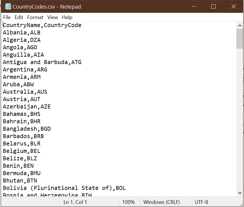
Open the file CountryCodes.txt in a text
editor. It will look like this:
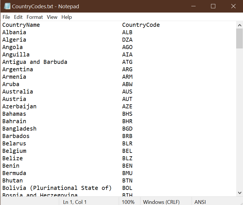
This is a fixed format file in which the CountryName variable starts on the 1st character of each line and the CountryCode variable starts on the 36th character.
To open this file in Excel, use the Text Import Wizard:
- Select
File > Open >from the menu. - Select
Browseto get to the usualOpenFiledialog box. - Find and select the file
CountryCodes.txt. You may need to move to the correct folder, and to change the file type to “All files (.)” - The first dialog box of the Text Import Wizard allows you to specify
the overall structure of your data file:
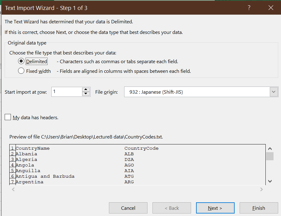 Excel guesses about the structure of your data, but you may need to
correct its guesses. In this case, you should change the file
type from
Excel guesses about the structure of your data, but you may need to
correct its guesses. In this case, you should change the file
type from DelimitedtoFixed width, and selectNext>.- Excel made a few other wrong guesses (it thinks that the file is written in Japanese!) but you can ignore them.
- The second dialog box of the Text Import Wizard allows you to
specify where each column starts:
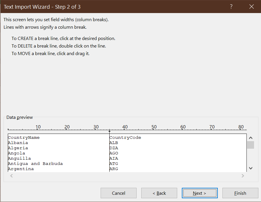
Excel seems to have guessed correctly in this case, so go ahead and selectNext>. - The final dialog box of the Text Import Wizard provides some
options for changing the data format for each individual column:
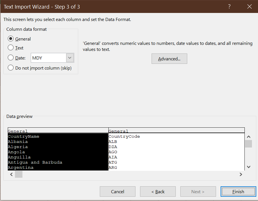
We do not need to worry about any of these options, so go ahead and selectFinish.
Our worksheet now contains the imported data, correctly arranged into cells. Keep this worksheet open.
10.1.2 CSV files
The most common and useful general-purpose format for tabular data is called the comma separated values or CSV file format. A CSV file is just a text file with the following features:
- Each line in the file represents a row in the table
- Within each row, cell values are separated or delimited by commas.
- Where necessary, text values are enclosed in quotes.
For example, this CSV file:
Name,Year of birth,Year of death
"Mary, Queen of Scots",1542,1547
Mary I,1516,1558
Elizabeth I,1533,1603
will appear in Excel as the table:
| Name | Year of birth | Year of death |
|---|---|---|
| Mary, Queen of Scots | 1542 | 1547 |
| Mary I | 1516 | 1558 |
| Elizabeth I | 1533 | 1603 |
Notice that the quotes around “Mary, Queen of Scots” are needed in order for the comma to be interpreted as an actual comma rather than a delimiter between cells.
Example 10.2 Exporting a CSV file from Excel
To save the Excel worksheet we created in the previous section as a CSV file:
- Select
File > Save As. You will see:- a text box giving the file name (
CountryCodes.txt) - a drop-down box giving the file format (
Text (Tab delimited) (*.txt)
- a text box giving the file name (
- Select
CSV (Comma delimited) (*.csv)from the drop-down box and - Enter a file name (I suggest CountryCodes.csv) in the text box.
- Select
Save.- You may get the warning message: The selected file type does
not support workbooks that contain multiple sheets. To save only
the active sheet click OK…. If so, select
OK.
- You may get the warning message: The selected file type does
not support workbooks that contain multiple sheets. To save only
the active sheet click OK…. If so, select
- Close Excel.
- You may get another warning message:
Want to save your changes to CountryCodes.csv?If so, selectDon't save.
- You may get another warning message:
You have created a CSV file.
You can see the exact contents of a CSV file by opening it in a text editor.
Example 10.3 Opening a CSV file as text
Use your preferred text editor to open the file CountryCodes.csv. It
will look something like this:
If a CSV file has .csv at the end of its file name, you can open it
in Excel by just double-clicking on it. Otherwise, you can use the
Text Import Wizard.
CSV files (and text files in general) have several important limitations
relative to regular Excel (.xlsx) files:
- A CSV file can only contain one table, while an Excel file can contain multiple tables.
- A CSV file can only contain cell values, and cannot contain:
- Formulas
- Formatting
- Graphs
- Any other fancy Excel features
These limitations are also the main advantage of the CSV file: they are simple ways of reporting tabular data and can be read by virtually any program, or even by a human.
10.1.3 Other file formats
In addition to CSV files, we will run into files that use characters other than the comma to delimit cells.
Space-delimited text files are just like CSV files, but use spaces as the delimiter. For example, a space-delimited version of our table might look like this:
Name "Year of birth" "Year of death"
"Mary, Queen of Scots" 1542 1547
"Mary I" 1516 1558
"Elizabeth I" 1533 1603
Tab-delimited text files are just like CSV files, but use a tab character as the delimiter.
Like fixed-width and CSV files, space-delimited and tab-delimited files can be imported into Excel using the Text Import Wizard.
Excel also has a wide variety of tools for obtaining data from various
databases, online services, etc. We do not have time to explore all of
these tools, but you can select Data from the menu bar and look
around to see what is available.
10.1.4 Text to columns
Sometimes you will run into an Excel sheet that looks like this:
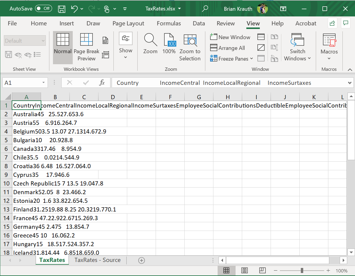
This can happen if a text file has been incorrectly imported, or if you have copied-and-pasted data from a PDF file or web page. Fortunately, Excel has a way of fixing that: the Text to Columns tool.
Example 10.4 Using the text-to-columns tool
Open the file TaxRates.xlsx. As you can see, it looks like the picture above. To use the Text to Columns tool:
- Select the column with the data (column A).
- Be sure to select the whole column, not just a single cell.
- Select
Data > Text to Columnsfrom the menu. - The Text to Columns Wizard will appear.
- It is very similar to the Text Import Wizard
- Excel is usually smart enough to guess the structure of your data and to offer the correct default options here.
- Assuming the default options are correct (you can see what
happens if you change the options), select
Next>, thenNext>again, thenFinish.
Your worksheet should now look like this:
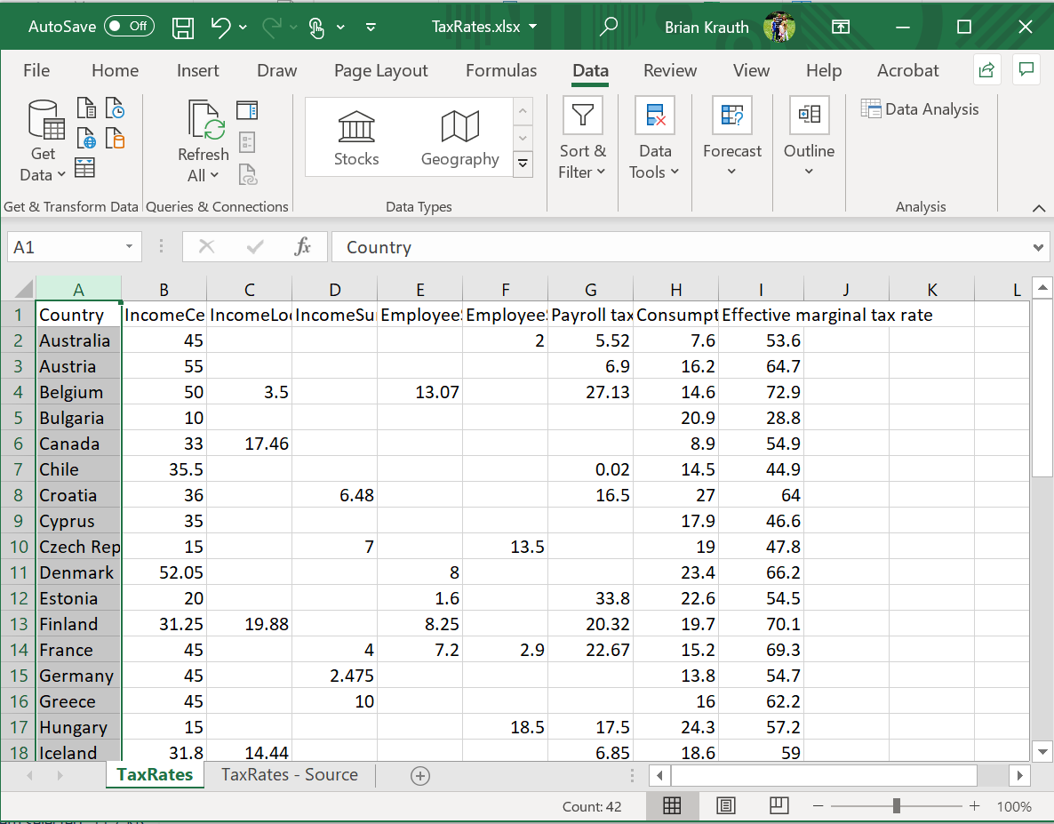
Save this file and exit Excel.
10.2 Combining data
The data that we wish to analyze often comes in multiple tables from multiple sources. In order to proceed with the analysis, we often need to combine information in various ways:
- We will want to combine multiple data files into a single Excel file.
- We will want to link observations in one table with observations in another table.
- We will want to construct new variables that are group-level aggregates (counts, averages, or sums) of existing variables.
This section will go through the most important tools and techniques of combining data in these ways.
10.2.1 Combining Excel files
Data tables often come in multiple files, especially if they are from different sources. It is possible for one Excel file to use data from another Excel file (or even a non-Excel file or online data source), but doing so can lead to problems if not done very carefully. For example, if one file has a formula that references another file, that formula may stop working if either file is moved to another folder.
An easier approach in most situations is to just combine everything into a single Excel workbook.
Example 10.5 Combining our cross-country data files
We currently have three data files: pwt100.xlsx, CountryCodes.csv, and TaxRates.xlsx. To combine them in a single file:
- Open all three files.
- Go to CountryCodes.csv, and right-click on the CountryCodes tab
at the bottom of the page. A menu will appear; select
Move or Copy...and theMove or Copydialog box will appear:
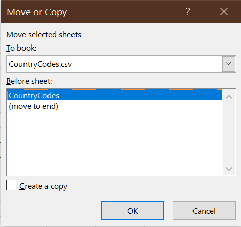
- Select pwt100.xslx from the
To book:drop-down box. Your worksheet will now move to that workbook. - Repeat the same process with both worksheets in the TaxRates.xlsx workbook.
- At this point all of our worksheets are in a single workbook. Save the workbook with name GrowthData.xlsx.
Before proceeding, it’s a good idea to make sure our data is tidy.
Example 10.6 Making the our workbook tidy
- Take a look at each of our three main worksheets and identify
if they need to be adjusted in any way to meet our criteria for
tidy data:
- CountryCodes is tidy and does not need alteration.
- TaxRates is tidy and does not need alteration.
- Data has one issue: each observation (row) appears to describe a particular country in a particular year. There is an identifier for country and an identifier for year, but no combined identifier that takes on a unique value for each individual observation. We will need to create one.
- Add a unique ID variable to the Data worksheet:
- Insert a new column to the left of the current column A.
- Enter CountryYear in cell A1 to name the variable.
- Use the
CONCAT()function to create the identifier in cell A2.- The formula would be
=CONCAT(B2,E2) - For example, if row 2 depicts Aruba (ABW) in 1950, cell A2 should display “ABW1950.”
- The formula would be
- Copy/paste or fill this formula to the rest of column A.
- Make a copy of the TaxRates worksheet, and name it GrowthData. This sheet will be the starting point for the linked data that we will construct in the next two sections.
Our data set is now tidy and ready to link.
10.2.2 Linking observations
One of the most common tasks in cleaning data is to combine variables from two or more data sets. In order to do this, we need to match or link observations in the two tables on the basis of one or more ID variables or keys.
All statistics packages have tools to link observations. In Excel,
the table you are obtaining data from is called a lookup table
and the key tool is the XLOOKUP() function:
- The
XLOOKUP()function takes three main/required arguments:- The
lookup_valueis the value in the current table to look up. - The
lookup_arrayis the range containing the column of IDs. - The
return_arrayis the range containing the column of values to return.
- The
For example, the formula =XLOOKUP("California",A1:A10,C1:C10) looks
for a row/observation with the value “California” in column A (cells A1:A10),
and then returns the value in column C (cells C1:C10) for that row/observation.
Example 10.7 Adding country codes to the tax rate data
The TaxRates worksheet from the Tax Foundation and the Data worksheet from the Penn World Table both provide information at the country level. But they do not yet have a common key variable:
- Data provides two ways of identifying a country in each observation:
- The country name
- The three-letter ISO country code.
- TaxRates only provides the country name.
We could try to match on country name, but the country names are not exactly the same in the two tables. For example, the same country is called “South Korea” in TaxRates and “Republic of Korea” in Data. This is a common problem with names, so people who work with data usually prefer standardized codes.
One option is to simply change the country names in one of our tables, but that goes against our general principle that we avoid changing data. A better solution is to use a crosswalk table that gives the country code for each country name, including name variations like “Republic of Korea” and “South Korea.” The CountryCodes worksheet is a crosswalk table I have created for this purpose. If you take a look at it, you will notice that there are observations for both “Republic of Korea” and “South Korea.”
Let’s use our crosswalk table and the XLOOKUP() function to add a country
code to the GrowthData worksheet.
- Insert a new column to the left of the current column A.
- You can do that by selecting any cell in column A, and then selecting
Home > Insert > Insert Sheet Columns
- You can do that by selecting any cell in column A, and then selecting
- Enter CountryCode in cell A1 to name the variable.
- Construct the appropriate formula in cell A2.
lookup_valueshould be the country name of the current observation (B2)lookup_arrayshould be the full list of country names (CountryCodes!A2:A185)return_arrayshould be the full list of country codes (CountryCodes!B2:B185)
- Change references in the formula from relative to absolute as appropriate. The
resulting formula will be
=XLOOKUP(B2,CountryCodes!A$2:A$185,CountryCodes!B$2:B$185) - Copy/paste or fill the formula to the remaining cells in column A.
Column A should now display the ISO country code for each observation.
XLOOKUP() can also be used to match on multiple criteria.
Example 10.8 Matching on multiple criteria
Now suppose we want to create a variable that is each country’s
population (pop in the Data worksheet) in 2019. Since
we need to match both country and year, we will need to use
the CONCAT() function to put the country and year together
in a single criterion.
- Enter Pop2019 in cell K1 of GrowthData to name the variable.
- Enter the correct formula in cell K2:
lookup_valueshould combine the country code (cell A2) with the year (2019), so it should beCONCAT(A2,"2019").lookup_arrayshould be the full range of the CountryYear variable in the Data worksheet (Data!A2:A12811).return_arrayshould be the full range of the pop variable in the Data worksheet (Data!H2:H12811).
- Make the cell references absolute where needed, which will result
in the formula
=XLOOKUP(CONCAT(A2,"2019"),Data!A$2:A$12811,Data!H$2:H$12811) - Copy/paste or fill the formula to the remaining cells in column
We can also create another variable whose variable is the country’s population in 1990.
- Enter Pop1990 in cell L1 of GrowthData to name the variable.
- Enter the correct formula in cell L2. It will be nearly identical
to the formula in cell K2, but with “2019” replaced by “1990”:
=XLOOKUP(CONCAT(A2,"1990"),Data!A$2:A$12811,Data!H$2:H$12811) - Copy/paste or fill the formula to the remaining cells in column
You may note that the PWT goes all the way back to 1950, and may wonder why I picked 1990 as my starting point. The reason for this is many countries do not have data going back to 1950, especially those countries that were part of or allied with the Soviet Union. By 1990, the PWT has data for almost all countries.
Normally, XLOOKUP() looks for an exact match and returns an error
if no match is found. This is a good default, but the optional
arguments if_not_found and match_mode can be used if you want
to do something other than that.
Related functions
XLOOKUP() is a relatively new addition to Excel, so you may see files that
use the older functions VLOOKUP() and HLOOKUP(). The syntax of these
functions is somewhat different, but the underlying idea is the same.
10.2.3 Aggregating by group
Sometimes we will want to create a new variable that is the sum or average of another variable within some group, or the count of the number of observations in that group.
We can construct group-level averages variables using the AVERAGEIFS()
function. It takes three arguments:
average_rangeis the range of cells containing the variable that should be averaged.criteria_rangeis the range of cells containing the group identifier variablecriteriais the cell containing the group identifier of the current observation.
For example =AVERAGEIFS(C1:C100,A1:A100,"California") returns the average
value in column C of all of the observations whose value in
column A is “California.”
Example 10.9 Average investment share by country
Suppose we are interested in whether high-tax countries tend to have higher or lower investment rates than low-tax countries. In order to do this, we might add a variable to our GrowthData worksheet that describes the average investment share of GDP (the variable csh_i) in each country over the full period of the data.
We can do this using the AVERAGEIFS() function:
- Enter AvgIShare in cell M1 to name the variable.
- Construct the correct formula in cell M2 using the function
AVERAGEIFS():average_rangeshould be the full range of investment shares (Data!AO2:AO12811)criteria_rangeshould be the full range of country codes (Data!A2:A12811)criteriashould be the cell containing the country code of the current observation (A2)
- Adjust the formula to have the correct absolute references. The
resulting formula should be
=AVERAGEIFS(Data!AO$2:AO$12811,Data!A$2:A$12811,A2) - Copy/paste or fill this formula into the remaining cells in column M.
The average investment share should range from a minimum of 0.13 for Bulgaria to a maximum of 0.44 for Cyprus.
The AVERAGEIFS() function is part of a family of functions that
calculate a statistic for a subset of observations that satisfy a
set of criteria:
COUNTIFS()calculates the number of observations meeting the criteria.- We used
COUNTIFS()to construct a frequency table in Chapter 6.
- We used
AVERAGEIFS()calculate the average of a variable for those observations that meet the criteria.SUMIFS()calculate the sum of a variable for those observations that meet the criteria.MINIFS()calculate the minimum of a variable for those observations that meet the criteria.MAXIFS()calculate the maximum of a variable for those observations that meet the criteria.
These functions can all be used to construct summary statistics (as in Chapter 6) or to construct group aggregate variables within our data set (as in this chapter).
Related functions
The COUNTIFS(), AVERAGEIFS(), SUMIFS(), MINIFS() and MAXIFS()
functions all allow for multiple criteria to be used. Excel also includes
a set of older functions COUNTIF(), AVERAGEIF(), SUMIF(),
MINIF() and MAXIF() that allow only a single criterion. You may
see these in older worksheets.
10.3 Advanced data management
10.3.1 Error codes
Sometimes an Excel formula does not produce a valid result. When that happens, Excel will return an error code to indicate what has gone wrong. Excel’s most commonly-used error codes are:
#VALUE!means you have given a function the wrong type of argument- Example:
=LN("THIS IS A STRING AND NOT A NUMBER")
- Example:
#NAME?means you have referenced a function that does not exist.- Example:
=NOTAREALFUNCTION(1)
- Example:
DIV/0!means you have divided by zero.- Example:
=1/0 - This error also appears when you take the
AVERAGE()of a range of cells that does no include any numbers.
- Example:
#REF!means you have referenced a cell that does not exist.- This usually happens when you delete a row or column that the formula refers to.
#NUM!means that the result of your numeric calculation is not a real number.- Example:
=SQRT(-1)
- Example:
#NAmeans that a lookup function such asXLOOKUP()was unable to find a match.
If you aren’t sure what an error code means, Google it.
Although error codes are helpful in figuring out what has gone wrong with a calculation, they should not be part of your final work product. Instead, you should rewrite your formulas to catch and handle error conditions.
Example 10.10 Catching and handling an error condition
Suppose you want the variable in column B to be the square root
of the variable in column A, but the variable in column A is sometimes
negative. As a result the simple formula =SQRT(A1) displays the
square root in some cases and the error code #NUM! in others.
We can use the IF() function to catch this error, and handle
it in whatever way we want. For example, the formula:
=IF(A1>=0,SQRT(A1),"")
will return the square root of A1 if A1 is positive or zero, and a
blank cell if A1 is negative.
10.3.2 Data validation
One potential source of errors is the entry of invalid data. Invalid data means that a particular cell in our data takes on a value that is not in the set of possible values for that variable. For example:
- A numeric variable has a non-numeric value.
- A logical variable has a value other than TRUE or FALSE.
- A date variable is in the wrong format.
- A text variable is the wrong length.
- A numeric variable is outside of its expected range, for example an unemployment rate of 200% or a negative value of GDP.
Invalid data can result from typos or other human error, or it can result from imperfect translation of data between different data sources.
Excel has a set of data validation tools to help prevent and fix
invalid data. Data validation can be accessed by selecting Data from
the menu and then clicking on the Data Validation button, which
looks like this:  .
.
Example 10.11 Adding data validation
The Pop2019 variable (column K in the GrowthData table) is a country’s population in 2019. Population cannot be negative, so let’s add this as a data validation requirement:
- Select column K in GrowthData.
- Select
Data > Data Validation. The Data Validation dialog box will appear:
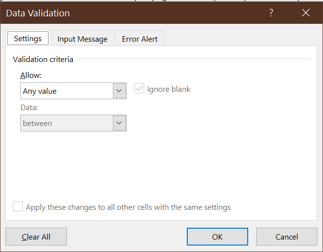
By default, it allows “Any value,” which means no restriction at all. - To add a restriction that negative values are not allowed:
- Select
Decimalfrom theAllowdrop-down box. - Select
greater than or equal tofrom theDatadrop-down box - Enter
0in theMinimumdrop-down box.
- Select
- Select
OK.
Although nothing appears to have changed, column K is now subject to data validation.
Once we have added data validation to a range of cells, several things will happen. First, Excel will not allow you to enter invalid data into a cell with validation turned on. This feature will help avoid problems in the first place.
Example 10.12 Entering invalid data
Go to cell K43, and (try to) enter -1. You will see this dialog
box telling you that this is an invalid value:
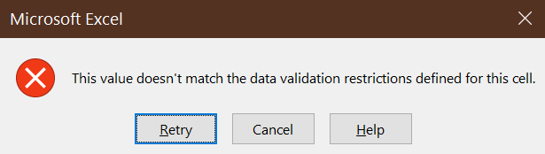
Select Cancel.
The Data Validation tool also allows you to identify previously-entered observations with invalid data.
Example 10.13 Finding invalid data
All of our Pop2019 data is valid, so in order to “find” invalid data we will need to cheat a little.
- Select column K again.
- Select
Data > Data Validationagain. - Change the Minimum value from “0” to “10.”
This will cause all values of Pop2019 below 10 to be (incorrectly) considered invalid.
To identify invalid observations, select
Data > Data Validation > Circle Invalid Data. You will now
see red circles around all values that violate the validation
criteria (there may be a slight delay):
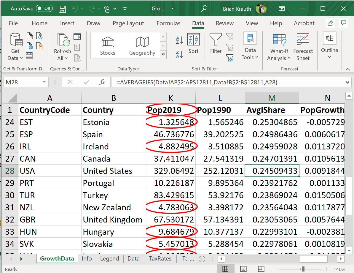
To remove the circles, select Data > Data Validation > Clear Validation Circles.
Finally, we can remove all data validation from a cell.
Example 10.14 Removing data validation
To remove data validation from the Pop2019 variable:
- Select column K in GrowthData.
- Select
Data > Data Validation. The Data Validation dialog box will appear. - Select
Clear Alland thenOK.
You can confirm that data validation has been removed by entering an invalid value (Excel will now let you do this) or by adding validation circles (there will not be any).
10.3.3 Protecting data
One of the most common Excel problems occurs when someone who is analyzing a data set unintentionally changes the data.
- This can happen because you accidentally touch your keyboard and overwrite the contents of a cell.
- It can also happens when an inexperienced analyst breaks the rule about keeping the original data untouched, and makes a mistake.
This is to some extent an unavoidable consequence of Excel’s fundamental design: there is no separation between data and analysis. This design feature has the positive implication that your data is always visible and accessible, but it comes at a cost.
One way of avoiding this cost is to make a practice of making your original data “read only.” Excel does this through the combined mechanisms of protecting sheets and locking cells.
- Each worksheet is either protected or unprotected.
- By default, all worksheets are unprotected.
- You can change the status of any worksheet.
- Each cell is either locked or unlocked.
- By default, all cells are locked.
- You can change the status of a cell or cell range.
- Any locked cell in any protected sheet cannot be edited.
Example 10.15 Protecting an entire worksheet
The PWT data table Data contains original raw that we do not want changed. To prevent changes to that worksheet:
- Right-click on the Data tab at the bottom of the page. A menu will appear.
- Select
Protect Sheet. The Protect Sheet dialog box will provide several options:
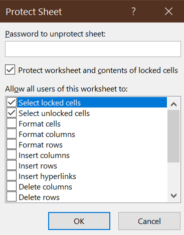
- Select
OK.
Now that you have protected the Data worksheet, try to edit any cell. You will get an error message.
In many cases, you will only want to protect certain cells in a given sheet. To do this, remember the rules: all cells are initially locked and all worksheets are unprotected. So we will need to unlock all cells except the ones we want locked, and then protect the sheet.
Example 10.16 Protecting part of a worksheet
To protect and lock columns A through N in GrowthData but keep the other columns unlocked:
- Select all of the cells in the worksheet by clicking on the
 button.
 - Unlock all of the cells by selecting
Home > Format > Lock Cell. - Lock columns A through N by selecting them, and then
selecting
Home > Format > Lock Cell. - Protect the worksheet by selecting
Home > Format > Protect Sheet - The
Protect Sheetdialog box will appear; selectOK.
Note that you have to do it in this order - Excel will not let you unlock locked cells after you have protected the sheet.
You will now get an error message if you try to edit any of the locked cells, but you can edit the unlocked cells in any way you like.
Finally, you can remove protection from any worksheet by simply
selecting Home > Format > Unprotect Sheet.
You can download the complete Excel file with all data cleaning from this chapter at https://bookdown.org/bkrauth/BOOK/sampledata/GrowthData.xlsx
10.4 Reading and viewing data in R
Before doing any statistical or graphical analysis, we need to get the data into R. We will also want to look at our data before diving into the analysis, and we may want to do some data cleaning as well.
We will use numerous Tidyverse functions, so we need to load the Tidyverse package:
# Load the tidyverse
library("tidyverse")
We will work with the employment data.
10.4.1 Reading a CSV file
Our first step will be reading the data in from the CSV file. The Tidyverse
function to do this is called read_csv(). It has one required argument:
the name of the CSV file.
- Ye can access the online data set directly in R.
- If you have a slow connection or want to work offline, you can download the data set from https://bookdown.org/bkrauth/BOOK/sampledata/EmploymentData.csv and then access the local data set.
# The code below accesses the online data.  You can also download the file
# 'EmploymentData.csv' and change the argument to read_csv() to the local file
# location
EmpData <- read_csv("https://bookdown.org/bkrauth/BOOK/sampledata/EmploymentData.csv")
## Rows: 541 Columns: 11
## -- Column specification --------------------------------------------------------
## Delimiter: ","
## chr (3): MonthYr, Party, PrimeMinister
## dbl (8): Population, Employed, Unemployed, LabourForce, NotInLabourForce, Un...
##
## i Use `spec()` to retrieve the full column specification for this data.
## i Specify the column types or set `show_col_types = FALSE` to quiet this message.
As you can see, R guesses each variable’s data type, and reports its guess. It is always a good idea to read this output and make sure that everything is the way that we want it:
- The numeric variables are all stored as
col_double().- This means double-precision (64 bit) real number
- This is what we want.
- The two text variables are both stored as
col_character().- This means character or text string
- This is what we want.
- The MonthYr variable is also stored as
col_character().- This is not what we want.
- We will want MonthYr to be stored explicitly as a date variable, so we make a note of that issue here and will fix it later.
- This is not what we want.
We have assigned the data in the CSV file to the variable EmpData.
Additional options
Our data file happens to be a nice and tidy one, so read_csv() worked
just fine with its default options. Not all data files are so
tidy, so read_csv() has many optional arguments. There are
also functions for other delimited file types:
read_csv2()for files delimited by semicolons rather than commasread_tsv()for tab-delimited filesread_delim()for files delimited using any other character
Base R function has a similar function called read.csv(),
but read_csv() is preferable for various reasons.
10.4.2 Viewing a data table
The read_csv() function creates an object called a tibble. A
tibble is a Tidyverse object type that describes a tidy data table.
- Each row in the tibble represents an observation
- Each column represents a variable, and has a name.
The base R equivalent of a tibble is called a data frame. Tibbles
and data frames are interchangeable in most applications, but
tibbles have some additional features that make them work better
with the Tidyverse.
We have several ways of viewing the contents of a tibble. We can start with the print function, which we have already seen in other contexts:
print(EmpData)
## # A tibble: 541 x 11
##    MonthYr   Population Employed Unemployed LabourForce NotInLabourForce UnempRate
##    <chr>          <dbl>    <dbl>      <dbl>       <dbl>            <dbl>     <dbl>
##  1 1/1/1976      16852.    9637.       733       10370.            6483.    0.0707
##  2 2/1/1976      16892     9660.       730       10390.            6502.    0.0703
##  3 3/1/1976      16931.    9704.       692.      10396.            6535     0.0665
##  4 4/1/1976      16969.    9738.       713.      10451.            6518.    0.0682
##  5 5/1/1976      17008.    9726.       720       10446.            6562     0.0689
##  6 6/1/1976      17047.    9748.       721.      10470.            6577.    0.0689
##  7 7/1/1976      17086.    9760.       780.      10539.            6546.    0.0740
##  8 8/1/1976      17124.    9780.       744.      10524.            6600.    0.0707
##  9 9/1/1976      17154.    9795.       737.      10532.            6622.    0.0699
## 10 10/1/1976     17183.    9782.       783.      10565.            6618.    0.0741
## # ... with 531 more rows, and 4 more variables: LFPRate <dbl>, Party <chr>,
## #   PrimeMinister <chr>, AnnPopGrowth <dbl>
Tibbles can be quite large, so the print() function will usually
show an abbreviated version of the table.
We can also see the whole table by executing the command View(EmpData) or
through RStudio:
- Go to the Environment tab in the upper right window.
- You will see a list of all variables currently in memory, including EmpData.
- Double-click on
EmpData.
You will see a spreadsheet-like display of EmpData. As in Excel, you can sort
and filter this table. Unlike Excel, you cannot edit it here.
10.4.3 Data table properties
There are several R functions available for exploring the properties of a data table.
We can obtain the column names of a tibble using the names() function:
names(EmpData)
##  [1] "MonthYr"          "Population"       "Employed"         "Unemployed"
##  [5] "LabourForce"      "NotInLabourForce" "UnempRate"        "LFPRate"
##  [9] "Party"            "PrimeMinister"    "AnnPopGrowth"
and we can count the rows and columns with nrow() and ncol() respectively:
nrow(EmpData)
## [1] 541
ncol(EmpData)
## [1] 11
We can access any variable by name using the $ notation:
length(EmpData$UnempRate)
## [1] 541
As you can see, the length() function returns the length of a vector.
Chapter review
In this chapter, we learned about many loosely-related topics. The underlying theme that connects them all is that real data can be complicated. We will often need to get data from multiple sources and in varying formats, and we cannot trust either ourselves or others not to make mistakes. So we need to be both disciplined in handling our data, and flexible in finding solutions to the problems that pop up.
In the next two chapters, we will develop more advanced methods for data analysis in both Excel and R.
Practice problems
Answers can be found in the appendix.
SKILL #1: Identify common data file formats
- Identify each of these text files as fixed-width, tab/space separated, or CSV
format.
Name   Age
Al     25
Betty  32
Name Age Al 25 Betty 32Name,Age Al,25 Betty,32
SKILL #2: Explain and implement common data cleaning tasks
- What is the purpose of each of the following:
- A crosswalk table
- Matching observations by keys
- Aggregating data by groups
SKILL #3: Describe and use Excel data management tools
- Under which of these scenarios can you edit cell A1?
- You open a blank sheet.
- You open a blank sheet, and protect the sheet.
- You open a blank sheet, unlock cells A1:C9 and protect the sheet.
- You open a blank sheet, lock cells A1:C9 and protect the sheet.
- What will happen if you:
- Add data validation to a column that contains invalid data.
- Add data validation to a column, and then try to enter invalid data
SKILL #4: Import and view data in R
- Use R (with the Tidyverse loaded) to open the data file https://people.sc.fsu.edu/~jburkardt/data/csv/deniro.csv and count the number of observations and variables in it.
I should mention that the Tax Foundation is not an entirely neutral organization - it generally supports lower taxes - and so my use of their data here should not be taken as expressing an opinion on their policy views. It is not unusual for useful data to come from politically-motivated sources; for many years the best data on tobacco prices and taxes came from the Tobacco Institute, a tobacco industry lobbying group (https://en.wikipedia.org/wiki/Tobacco_Institute).↩︎