Chapter 5 More on random variables

The previous chapter developed the basic terminology and analytical tools for a single discrete random variable. This chapter will extend those tools to work wit continuous random variables, and with multiple random variables.

Chapter goals

In this chapter we will:

Interpret the CDF and PDF of a continuous random variable.
Work with common continuous probability distributions including the uniform and normal.
Calculate and interpret joint, marginal and conditional distributions of two random variables.
Calculate and interpret the covariance and correlation coefficient of two discrete random variables.

5.1 Continuous random variables

So far we have considered random variables with a discrete support. However, many random variables of interest have a continuous support.

For example, consider the Canadian labour force participation rate. It is defined as: \[(\textrm{LFP rate}) = \frac{(\textrm{labour force})}{(\textrm{population})} \times 100\%\] so it can be any (rational) number between 0% and 100%: \[S_{LFP rate} = [0\%,100\%]\] This introduces a complication: there is an infinite number of values in this support. There is even an infinite number of possible values between two much closer numbers like 63% and 63.0001%.

Because a continuous random variable has an infinite support, it has a seemingly inconsistent pair of properties:

The probability that $x$ is any specific value in the support is: \[\Pr(x = a) = 0\] for all $a \in S_x$.
The probability that $x$ is somewhere in the support is: \[\Pr(x \in S_x) = 1\]

This feature applies to ranges as well. For example, the Canadian labour force participation rate has a high probability of being between 60% and 70%, but zero probability of being exactly 65%.

The math for working with continuous random variables is a little different from the math for working with discrete random variables, and is harder because it requires calculus. In many cases, it requires integral calculus (MATH 152 or MATH 158) which is not a prerequisite to this course, and which I do not expect you to know.

But deep down, there are no really important differences between continuous and discrete random variables. The intuition for why is straightforward: you can make a continuous random variable into a discrete random variable by just rounding it. For example, suppose you round the labour force participation rate to the nearest percentage point. Then it becomes a discrete random variable, with support: \[S_x = \{0\%, 1\%, \ldots 99\%, 100\% \}\] The same point applies if you round to the nearest 1/100th of a percentage point, or the nearest 1/1,000,000th of a percentage point.

Since discrete and random variables are more alike than first appears, most of the results and intuition we have already developed for discrete random variables can also be applied to continuous random variables. So:

Most of my examples will be for discrete case.
I will briefly show you the math for the continuous case, but I will not expect you to do it.
Most of the results I give you will apply for both cases.

Any time you see an integral here, you can ignore it.

5.1.1 The continuous CDF

The CDF of a continuous random variable $x$ is defined exactly the same way as for the discrete case: \[F_x(a) = \Pr(x \leq a)\] The only difference is how it looks.

If you recall, the CDF of a discrete random variable takes on a stair-step form: increasing in discrete jumps at every point in the discrete support, and flat everywhere else.

In contrast, the CDF of a continuous random variable increases continuously. It can have flat parts, but never jumps.

Example 5.1 The standard uniform distribution

Consider a random variable $x$ that has the standard uniform distribution. What that means is that:

The support of $x$ is the range $[0,1]$.
All values in this range are equally likely.

The CDF of the standard uniform distribution is: \[F_x(a) = \Pr(x \leq a) = \begin{cases} 0 & a < 0 \\ a & a \in [0,1] \\1 & a > 1 \\ \end{cases}\] Figure 5.1 below shows the CDF of the standard uniform distribution.

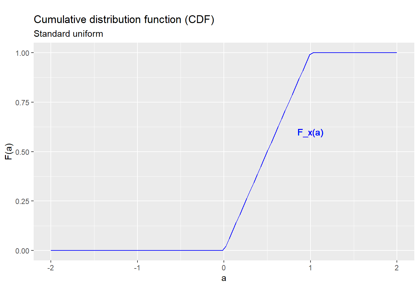
Figure 5.1: CDF for the standard uniform distribution

As you can see, the CDF is smoothly increasing between zero and one, and flat everywhere else.

The CDF of a continuous random variable obeys all of the properties described in section 4.1.4:

\[F_x(a) \leq F_x(b) \qquad \textrm{ if $a \leq b$} \] \[0 \leq F_x(a) \leq 1\] \[\lim_{a \rightarrow -\infty} F_x(a) = \Pr(x \leq -\infty) = 0\] \[\lim_{a \rightarrow \infty} F_x(a) = \Pr(x \leq \infty) = 1\] \[\begin{align} F(b) - F(a) &= \Pr(a < x \leq b) \end{align}\] In addition, the result on intervals applies to both strict and weak inequalities: \[\begin{align} F(b) - F(a) &= \Pr(a < x \leq b) \\ &= \Pr(a < x < b) \\ &= \Pr(a \leq x \leq b) \\ &= \Pr(a \leq x < b) \end{align}\] since a continuous random variable has probability zero of taking on any specific value.

5.1.2 The continuous PDF

The PDF $f_x(a)$ for a discrete random variable is defined as the size of the “jump” in the CDF at $a$, or (equivalently) the probability $\Pr(x=a)$ of observing that particular value. But the CDF of a continuous random variable has no jumps, and the probability of observing any particular value is always zero. So this particular function is useless in describing the probability distribution of a continuous random variable.

Instead, we define the PDF of a continuous random variable $x$ as the slope or derivative of the CDF: \[f_x(a) = \frac{d F_x(a)}{da}\] In other words, instead of the amount the CDF increases (jumps) at $a$, it is the rate at which it increases.

Example 5.2 The PDF of the standard uniform distribution

The PDF of a standard uniform random variable is: \[f_x(a) = \begin{cases} 0 & a < 0 \\ 1 & a \in [0,1] \\ 0 & a > 1 \\ \end{cases}\] which looks like this: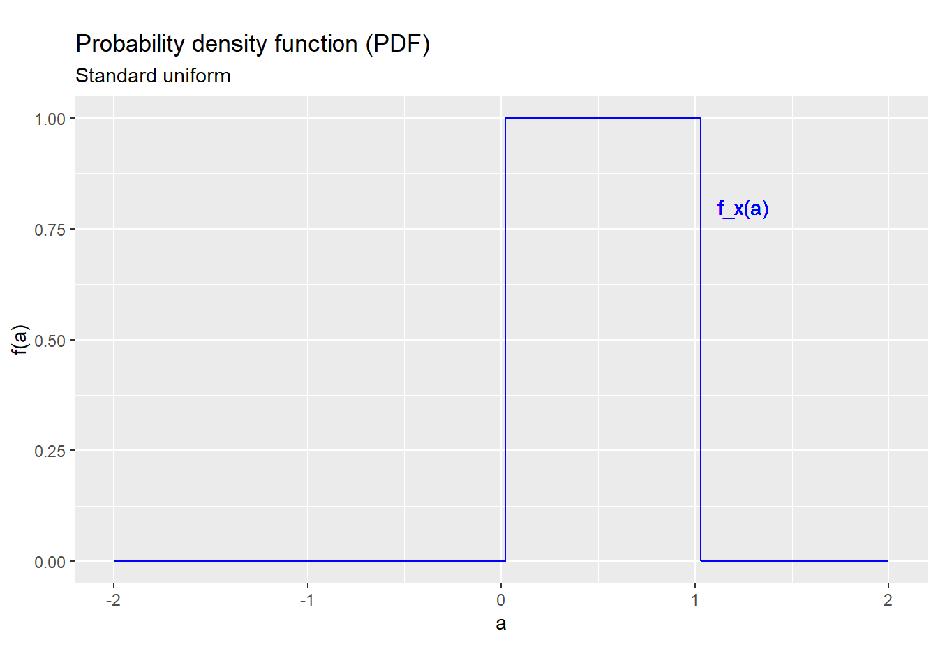

Figure 5.2: PDF for the standard uniform distribution

The PDF of a continuous random variable is a good way to visualize its probability distribution, and this is about the only way we will use the continuous PDF in this class (since everything else requires integration).

Example 5.3 Interpreting the uniform PDF

The uniform PDF shows the key feature of this distribution: in some loose sense, all values in the support are “equally likely,” much like in the discrete uniform distribution described earlier. In fact, if you round a uniform random variable, you get a discrete uniform random variable.

I have defined the PDF in terms of the CDF, but it is also possible to derive the CDF from the PDF. This requires integral calculus, so I will give the definition below but not expect you to use it.

Deriving the CDF from the PDF of a continuous random variable

The formula for deriving the CDF of a continuous random variable from its PDF is: \[F_x(a) = \int_{-\infty}^a f_x(v)dv\] Unless you have taken MATH 152 or MATH 158, you may have no idea what this is or how to solve it. That’s OK! All you need to know for this course is that it can be solved.

The continuous PDF has many properties that are similar but not identical to the properties of the discrete PDF.

Like the discrete PDF, the continuous PDF is non-negative for all values: \[f_x(a) \geq 0\] and is strictly positive for all values in the support: \[a \in S_x \implies f_x(a) > 0\] but it is not a probability, and can be greater than one.

If you recall, we can calculate probabilities from the discrete PDF by adding, and the discrete PDF sums to one. Similarly, we can calculate probabilities from the continuous PDF by integrating: \[\Pr(a < x < b) = \int_a^b f_x(v)dv\] and the continuous PDF integrates to one: \[\int_{-\infty}^{\infty} f_x(v)dv = 1\]

5.1.3 Means and quantiles

Quantiles and percentiles, including the range and median, have the same definition and interpretation whether the random variable is continuous or discrete.

The definition for the expected value of a continuous random variable is different and uses integral calculus.

The expected value for a continuous random variable

When $x$ is continuous, its expected value is defined as: \[E(x) = \int_{-\infty}^{\infty} af_x(a)da\] Notice that this looks just like the definition for the discrete case, but with the sum replaced by an integral sign. If you know much about integral calculus, you may require that an integral is a sum (or more precisely, the limit of a sum). This is why the same properties we earlier found for the expected value of a discrete random variable also applies to continuous random variables.

There is even a general definition that covers both discrete and continuous variables, as well as any mix between them: \[E(x) - \int_{-\infty}^{\infty} a dF_x(a)\] This expression uses notation that is not typically taught in a first course in integral calculus, so even if you have taken MATH 152 or MATH 158 you may not know how to interpret it. Again, I am only showing you so that you know the formula exists, I am not asking you to remember or use it.

More importantly, the expected value has the same interpretation as it does for a discrete random variable, and it has all of the properties described earlier as well.

The variance and standard deviation are both defined as expected values, so they also have the same interpretation and properties for a continuous random variable as they do for a discrete random variable.

5.2 The uniform distribution

The uniform probability distribution is usually written \[x \sim U(L,H)\] where $L < H$.

5.2.1 The uniform PDF

The uniform distribution is a continuous probability distribution with support: \[S_x = [L,H]\] and PDF: \[f_x(a) = \begin{cases}\frac{1}{H-L} & a \in S_x \\ 0 & \textrm{otherwise} \\ \end{cases}\]

For example, if $x \sim U(2,5)$ its support is the range of all values from 2 to 5, and its PDF looks like this: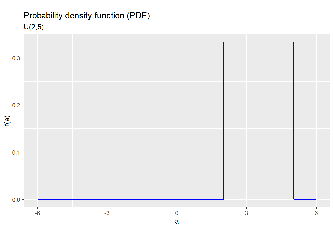

Figure 5.3: PDF for the U(2,5) distribution

The uniform distribution puts equal probability on all values between $L$ and $H$. We have already seen the standard uniform distribution, which is just the $U(0,1)$ distribution.

5.2.2 The uniform CDF

The CDF of the $U(L,H)$ distribution is \[F_x(a) = \begin{cases} 0 & a \leq L \\ \frac{a-L}{H-L} & L < a < H \\ 1 & a \geq H \\ \end{cases}\] For example, if $x \sim U(2,5)$ the CDF looks like this: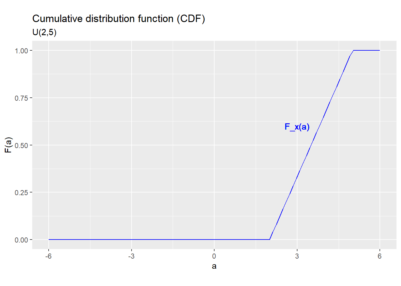

Figure 5.4: CDF for the U(2,5) distribution

5.2.3 Means and quantiles

The median of a uniform random variable $x \sim U(L,H)$ is just the midpoint of its support: \[Med(x) = F_x^{-1}(0.5) = \frac{L+H}{2}\] Its mean can be found using integral calculus, and is also the midpoint: \[E(x) = \frac{L+H}{2}\] Its variance also requires integral calculus: \[var(x) = \frac{(H-L)^2}{12}\] and its standard deviation is just the square root of the variance: \[sd(x) = \sqrt{\frac{(H-L)^2}{12}}\] as always.

5.2.4 Functions of a uniform

A linear function of a uniform random variable also has a uniform distribution. That is, if $x \sim U(L,H)$ and $y = a + bx$ where $b > 0$, then: \[y \sim U(a + bL, a + bH)\] A nonlinear function of a uniform random variable is generally not uniform, but it has a very useful characteristic described below.

Uniform distributions in video games

Uniform distributions are important in many computer applications including video games.

It is easy for a computer to generate a random number from the $U(0,1)$ distribution, and a $U(0,1)$ has the unusual feature that its $q$ quantile is equal to $q$.

As a result, you can generate a random variable with any probability distribution you like by following these steps:

Generate a random variable $q \sim U(0,1)$.
Calculate $x = F^{-1}(q)$ where $F(\cdot)$ is the CDF of the distribution you want.

Then $x$ is a random variable with the CDF $F(\cdot)$

If you have ever played a video game, that game is constantly generating $U(0,1)$ random numbers and using them to determine the behavior of non-player characters, the location of weapons and other resources, etc. Without that element of randomness, these games would be far too predictable to be much fun.

5.3 The normal distribution

The normal distribution is typically written as: \[ x \sim N(\mu,\sigma^2)\] The normal distribution is also called the Gaussian distribution, and the $N(0,1)$ distribution is called the standard normal distribution.

5.3.1 The normal PDF

The $N(\mu,\sigma^2)$ distribution is a continuous distribution with support $S_x = \mathbb{R}$ and PDF: \[f_x(a) = \frac{1}{\sigma \sqrt{2\pi}} e^{-\frac{(a-\mu)^2}{2\sigma}}\]

For example, the PDF for the $N(0,1)$ distribution looks like this: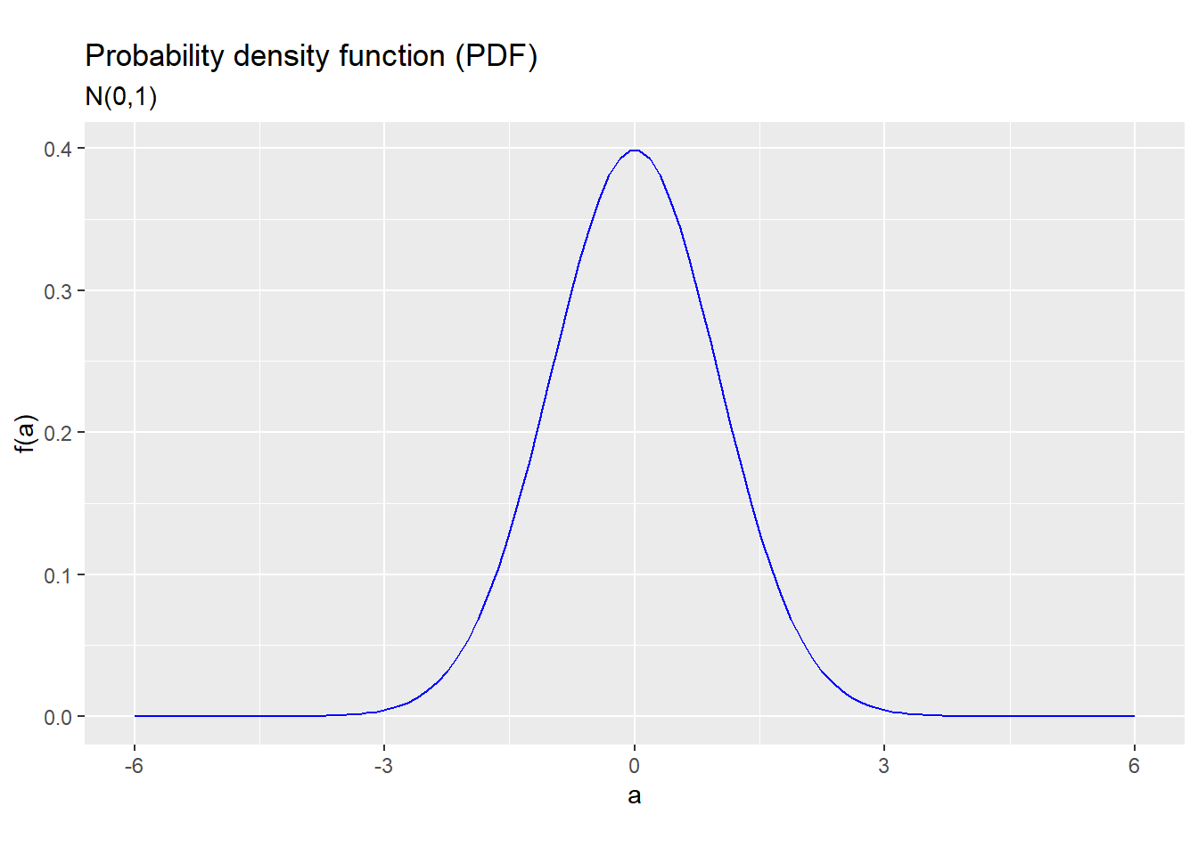

Figure 5.5: PDF for the N(0,1) distribution

As the figure shows, the $N(0,1)$ distribution is symmetric around $\mu=0$ and bell-shaped, meaning that it is usually close to zero but can occasionally be quite far.

For other values of $\mu$, the $N(\mu,\sigma^2)$ distribution is also symmetric around $\mu$ and bell-shaped, with the “spread” of the distribution depending on the value of $\sigma^2$: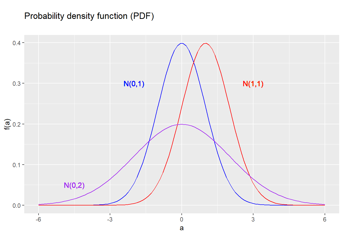

Figure 5.6: PDF for several normal distributions

5.3.2 The normal CDF

The CDF of the normal distribution can be derived by integrating the PDF. There is no simple closed-form expression for this CDF, but it is easy to calculate with a computer.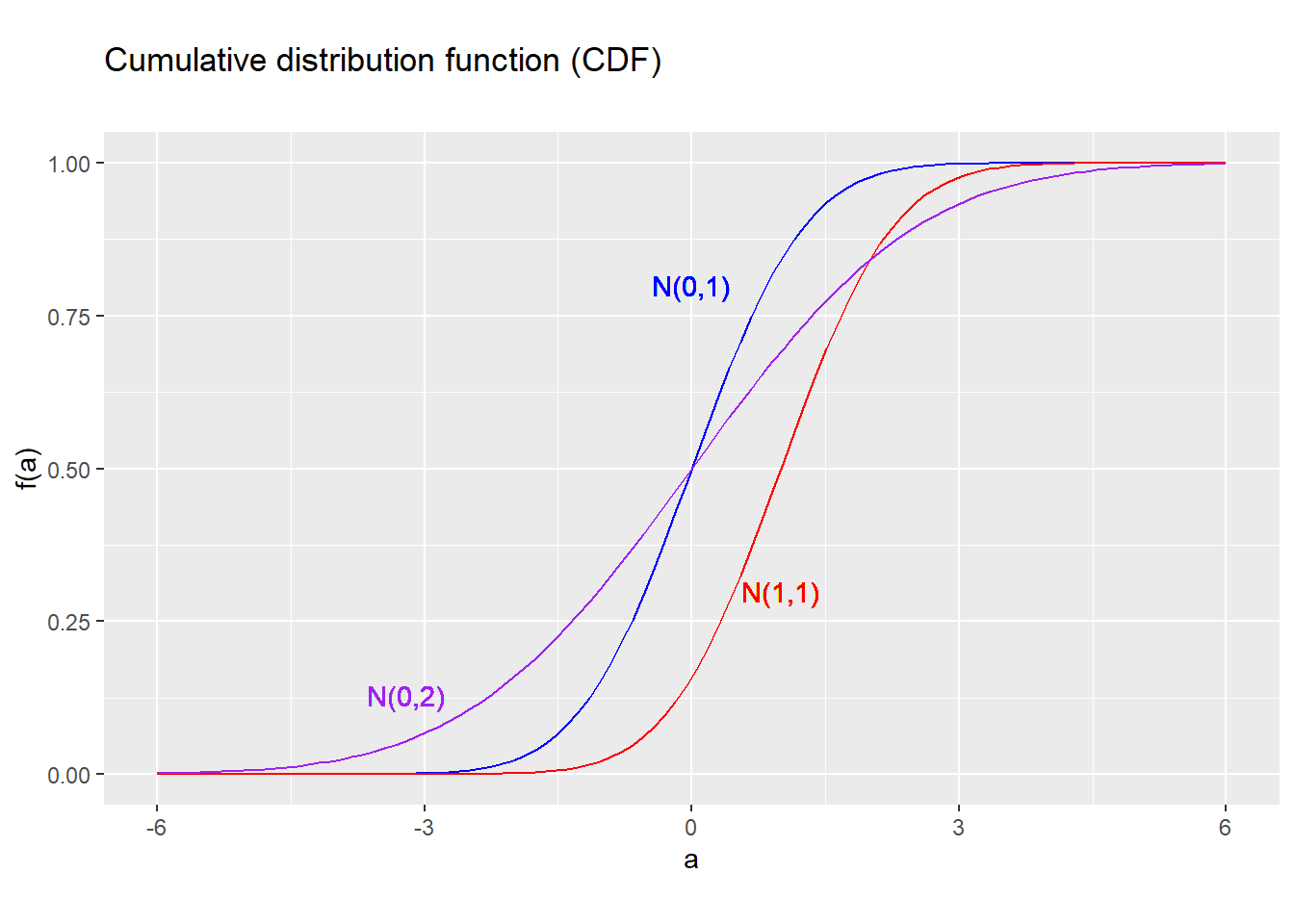

Figure 5.7: PDF for several normal distributions

The Excel function NORM.DIST() can be used to calculate the PDF or CDF of any normal distribution.

5.3.3 Means and quantiles

The Excel function NORM.INV() can be used to calculate the quantile (inverse CDF) function of any normal distribution.

Since the $N(\mu,\sigma^2)$ distribution is symmetric around $\mu$, its median is also $\mu$.

The mean and variance of a $N(\mu,\sigma^2)$ random variable can be found by integration: \[E(x) = \mu\] \[var(x) = \sigma^2\] and the standard deviation is just the square root of the variance: \[sd(x) = \sigma\]

5.3.4 Functions of a normal

Any linear function of a normal random variable is also normal. That is, if \[x \sim N(\mu,\sigma^2)\] Then for any constants $a$ and $b$: \[ax + b \sim N(a\mu + b, a^2\sigma^2)\] Just to be clear, we already showed that $E(ax +b) = aE(x) + b$ and $var(ax+b) = a^2 var(x)$ for any random variable $x$. What is new here is that $ax +b$ is normally distributed if $x$ is.

There are many other standard distributions that describe functions of one or more normal random variables and are derived from the normal distribution. These distributions include the $\chi^2$ distribution, the $F$ distribution and the $T$ distribution, and have various applications in statistical analysis.

5.3.5 The standard normal distribution

The standard normal distribution is so useful that we have special symbol for its PDF: \[\phi(a) = \frac{1}{\sqrt{2\pi}} e^{-\frac{a^2}{2}}\] and its CDF: \[\Phi(a) = \int_{-\infty}^a \phi(b)db\] All statistical programs, including Excel and R, provide a function that calculates the standard normal CDF.

Our result in the previous section about linear functions of a normal can be used to restate the distribution of any normally distributed random variable in terms of a standard normal. That is, suppose that \[x \sim N(\mu, \sigma^2)\] Then if we define \[z = \frac{x - \mu}{\sigma}\] our result implies that \[z \sim N\left(\frac{\mu-\mu}{\sigma}, \left(\frac{1}{\sigma}\right)^2 \sigma^2\right)\] or equivalently: \[z \sim N(0,1)\] We can use this result to derive the CDF of $x$: \[\begin{align} F_x(a) &= \Pr\left(x \leq a\right) \\ &= \Pr\left( \frac{x-\mu}{\sigma} \leq \frac{a-\mu}{\sigma}\right)\\ &= \Pr\left( z \leq \frac{a-\mu}{\sigma}\right) \\ &= \Phi\left(\frac{a-\mu}{\sigma}\right) \end{align}\] Since the standard normal CDF is available as a built-in function in Excel or R, so we can use this result to calculate the CDF for any normally distributed random variable.

A very important result called the Central Limit Theorem tells us that many “real world” random variables have a probability distribution that is well-approximated by the normal distribution.

We will discuss the central limit theorem in much more detail later.

5.4 Multiple random variables

Almost all interesting data sets have multiple observations and multiple variables. So before we start talking about data, we need to develop some tools and terminology for thinking about multiple random variables.

To keep things simple, most of the definitions and examples will be stated in terms of two random variables. The extension to more than two random variables is conceptually straightforward but will be skipped.

5.4.1 Joint distribution

Let $x = x(b)$ and $y = y(b)$ be two random variables defined in terms of the same underlying outcome $b$.

Their joint probability distribution assigns a probability to every event that can be defined in terms of $x$ and $y$, for example $\Pr(x = 6 \cap y = 0)$ or $\Pr(x < y)$.

This joint distribution can be fully described by the joint CDF: \[F_{x,y}(a,b) = \Pr(x \leq a \cap y \leq b)\] or by the joint PDF: \[f_{x,y}(a,b) = \begin{cases} \Pr(x = a \cap y = b) & \textrm{if $x$ and $y$ are discrete} \\ \frac{\partial F_{x,y}(a,b)}{\partial a \partial b} & \textrm{if $x$ and $y$ are continuous} \\ \end{cases}\]

Example 5.4 The joint PDF in roulette

In our roulette example, the joint PDF of $w_{red}$ and $w_{14}$ can be derived from the original outcome.

If $b=14$, then both red and 14 win: \[\begin{align} f_{red,14}(1,35) &= \Pr(w_{red}=1 \cap w_{14} = 35) \\ &= \Pr(b \in \{14\}) = 1/37 \end{align}\] If $b \in Red$ but $b \neq 14$, then red wins but 14 loses: \[\begin{align} f_{red,14}(1,-1) &= \Pr(w_{red} = 1 \cap w_{14} = -1) \\ &= \Pr\left(b \in \left\{ \begin{gathered} 1,3,5,7,9,12,16,18,19,21,\\ 23,25,27,30,32,34,36 \end{gathered}\right\}\right) \\ &= 17/37 \end{align}\] Otherwise both red and 14 lose: \[\begin{align} f_{red,14}(-1,-1) &= \Pr(w_{red} = -1 \cap w_{14} = -1) \\ &= \Pr\left(b \in \left\{ \begin{gathered} 0,2,4,6,7,10,11,13,15,17, \\ 20,22,24,26,28,31,33,35 \end{gathered}\right\}\right) \\ &= 19/37 \end{align}\] All other values have probability zero.

5.4.2 Marginal distribution

The joint distribution tells you two things about these variables

The probability distribution of each individual random variable, sometimes called that variable’s marginal distribution.
- For example, we can derive each variable’s CDF from the joint CDF: \[F_x(a) = \Pr(x \leq a) = \Pr(x \leq a \cap y \leq \infty) = F_{x,y}(a,\infty)\] \[F_y(b) = \Pr(y \leq b) = \Pr(x \leq \infty \cap y \leq b) = F_{x,y}(\infty,b)\]
- We can also derive each variable’s PDF from the joint PDF
The relationship between the two variables.
- We will develop several ways of describing this relationship: conditional distribution, covariance, correlation, etc.

Note that while you can always derive the marginal distributions from the joint distribution, you cannot go the other way around unless you know everything about the relationship between the two variables.

Example 5.5 Three joint distributions with identical marginal distributions

The scatter plots in Figure 5.8 below depict simulation results for a pair of random variables $(x,y)$, with a different joint distribution in each graph. In all three graphs, $x$ and $y$ have the same marginal distribution (standard normal).

The differences between the graphs are in the relationship between $x$ and $y$.

In the first graph, $x$ and $y$ are unrelated, so the data looks like as a “cloud” of random dots.
In the second graph, $x$ and $y$ have something of a negative relationship. High values of $x$ tend to go with low values of $y$.
In the third graph, $x$ and $y$ are positively and closely related. In fact, they are equal.

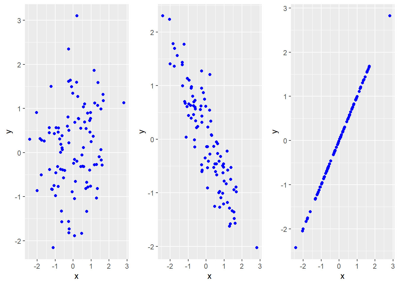
Figure 5.8: x and y have the same marginal distribution in all three graphs, but not the same joint distribution.

5.4.3 Conditional distribution

The conditional distribution of a random variable $y$ given another random variable $x$ assigns values to all probabilities of the form: \[\Pr(y \in A| x \in B) = \frac{\Pr(y \in A \cap x \in B)}{\Pr(x \in B)}\] Since a conditional probability is just the ratio of the joint probability to the marginal probability, the conditional distribution can always be derived from the joint distribution.

We can describe a conditional distribution with either the conditional CDF: \[F_{y|x}(a,b) = \Pr(y \leq a|x=b)\] or the conditional PDF \[f_{y|x}(a,b) = \begin{cases} \Pr(y=a|x=b) & \textrm{if $x$ and $y$ are discrete} \\ \frac{\partial}{\partial a}F_{y|x}(a,b) & \textrm{if $x$ and $y$ are continuous} \\ \end{cases} \]

Example 5.6 Conditional PDFs in roulette

Let’s find the conditional PDF of the payout for a bet on 14 given the payout for a bet on red. \[\begin{align} \Pr(w_{14}=-1|w_{red}=-1) &= \frac{\Pr(w_{14}=-1 \cap w_{red}=-1)}{\Pr(w_{red}=-1)} \\ &=\frac{19/37}{19/37} = 1 \\ \Pr(w_{14}=35|w_{red}=-1) &= \frac{\Pr(w_{14}=35 \cap w_{red}=-1)}{\Pr(w_{red}=-1)} \\ &=\frac{0}{19/37} = 0 \\ \Pr(w_{14}=-1|w_{red}=1) &= \frac{\Pr(w_{14}=-1 \cap w_{red}=1)}{\Pr(w_{red}=1)} \\ &= \frac{17/37}{18/37} \approx 0.944 \\ \Pr(w_{14}=35|w_{red}=1) &= \frac{\Pr(w_{14}=35 \cap w_{red}=1)}{\Pr(w_{red}=1)} \\ &= \frac{1/37}{18/37} \approx 0.056 \end{align}\]

5.4.4 Functions of multiple random variables

As with a single random variable, we can take any function $g(x,y)$ of two or more random variables, and we will have a new random variable that has a well-defined CDF, PDF, expected value, etc.

As with a linear function of a single random variable, we can take the expected value inside of a linear function of two or more random variables. That is: \[E(a + bx + cy) = a + bE(x) + cE(y)\] where $x$ and $y$ are random variables and $a$, $b$ and $c$ are constants.

However, we cannot take the expected value inside a nonlinear function. For example: \[E(xy) \neq E(x)E(y)\] \[E(x/y) \neq E(x)/E(y)\] As with a single random variable, the reason for this is that the expected value is a sum.

Example 5.7 Multiple bets in roulette

Suppose we bet $100 on red and $10 on 14. Our net payout will be: \[w_{total} = 100*w_{red} + 10*w_{14}\] which has expected value: \[\begin{align} E(w_{total}) &= E(100 w_{red} + 10 w_{14}) \\ &= 100 \, \underbrace{E(w_{red})}_{\approx -0.027} + 10 \, \underbrace{E(w_{14})}_{\approx -0.027} \\ &\approx -3 \end{align}\] That is we expect this betting strategy to lose an average of about $3 per game.

5.4.5 Covariance

The covariance of two random variables $x$ and $y$ is defined as: \[\sigma_{xy} = cov(x,y) = E[(x-E(x))*(y-E(y))]\] The covariance can be interpreted as a measure of how $x$ and $y$ tend to move together:

If the covariance is positive:
- $(x-E(x))$ and $(y-E(y))$ tend to have the same sign.
- $x$ and $y$ tend to move in the same direction.
If the covariance is negative:
- $(x-E(x))$ and $(y-E(y))$ tend to have opposite signs.
- $x$ and $y$ tend to move in opposite directions.

If the covariance is zero, there is no simple pattern of co-movement for $x$ and $y$.

Example 5.8 Calculating the covariance from the joint PDF

The covariance of $w_{red}$ and $w_{14}$ is: \[\begin{align} cov(w_{red},w_{14}) &= \begin{aligned}[t] & (1-\underbrace{E(w_{red})}_{\approx -0.027})(35-\underbrace{E(w_{14})}_{\approx -0.027})\underbrace{f_{red,14}(1,35)}_{1/37}\\ &+ (1-\underbrace{E(w_{red})}_{\approx -0.027})(-1-\underbrace{E(w_{14})}_{\approx -0.027})\underbrace{f_{red,14}(1,-1)}_{17/37} \\ &+ (-1-\underbrace{E(w_{red})}_{\approx -0.027})(-1-\underbrace{E(w_{14})}_{\approx -0.027})\underbrace{f_{red,14}(-1,-1)}_{19/37} \\ \end{aligned} \\ &\approx 0.999 \end{align}\] That is, the returns from a bet on red and a bet on 14 are positively related.

As with the variance, we can derive an alternative formula for the covariance: \[cov(x,y) = E(xy) - E(x)E(y)\] The derivation of this result is as follows: \[\begin{align} cov(x,y) &= E((x-E(x))(y-E(y))) \\ &= E(xy - yE(x) - xE(y) + E(x)E(y)) \\ &= E(xy) - E(y)E(x) - E(x)E(y) + E(x)E(y)) \\ &= E(xy) - E(x)E(y) \end{align}\] Again, this formula is often easier to calculate than using the original definition.

Example 5.9 Another way to calculate the covariance

The expected value of $w_{red}w_{14}$ is: \[\begin{align} E(w_{red}w_{14}) &= \begin{aligned}[t] & 1*35*\underbrace{f_{red,14}(1,35)}_{1/37}\\ &+ 1*(-1)*\underbrace{f_{red,14}(1,-1)}_{17/37} \\ &+ (-1)*(-1)*\underbrace{f_{red,14}(-1,-1)}_{19/37} \\ \end{aligned} \\ &= 35/37 - 17/37 + 19/37 \\ &= 1 \end{align}\] So the covariance is: \[\begin{align} cov(w_{red},w_{14}) &= E(w_{red}w_{14}) - E(w_{red})E(w_{14}) \\ &= 1 - (-0.027)*(-0.027) \\ &\approx 0.999 \end{align}\] which is the same result as we calculated earlier.

The key to understanding the covariance is that it is the expected value of a product $(x-E(x))(y-E(y))$, and the expected value itself is just a sum.

The first implication of this insight is that the order does not matter: \[cov(x,y) = cov(y,x)\] since $x*y = y*x$

A second implication is that the variance is just the covariance of a random variable with itself: \[cov(x,x) = var(x)\] since $x*x = x^2$.

Next, we can use our previous results on the expected value of a linear function of one or more random variables to derive some results on the covariance:

Covariances pass through sums: \[cov(x,y+z) = cov(x,y) + cov(x,z)\]
Constants can be taken out of covariances: \[cov(x,a+by) = b \, cov(x,y)\]

These results can be combined in various ways, for example: \[\begin{align} var(x + y) &= cov(x + y, x + y) \\ &= cov(x + y, x) + cov(x + y,y) \\ &= cov(x,x) + cov(y, x) + cov(x,y) + cov(y,y) \\ &= var(x) + 2 \, cov(x,y) + var(y) \\ \end{align}\] I do not expect you to remember all of these formulas, but be prepared to see me use them

5.4.6 Correlation

The correlation coefficient of two random variables $x$ and $y$ is defined as: \[\rho_{xy} = corr(x,y) = \frac{cov(x,y)}{\sqrt{var(x)var(y)}} = \frac{\sigma_{xy}}{\sigma_x\sigma_y}\] Like the covariance, the correlation describes the strength of a (linear) relationship between $x$ and $y$. But it is re-scaled in a way that makes it more convenient for some purposes.

Example 5.10 Correlation in roulette

The correlation of $w_{red}$ and $w_{14}$ is: \[\begin{align} corr(w_{red},w_{14}) &= \frac{cov(w_{red},w_{14})}{\sqrt{var(w_{red})*var(w_{14})}} \\ &\approx \frac{0.999}{\sqrt{1.0*34.1}} \\ &\approx 0.17 \end{align}\]

The covariance and correlation always have the same sign since standard deviations are always⁵ positive. The key difference between them is that correlation is scale-invariant. That is:

It always lies between -1 and 1.
It is unchanged by any re-scaling or change in units. That is, for any positive constants $a$ and $b$: \[corr(ax,by) = corr(x,y)\]

When $corr(x,y) \in \{-1,1\}$, then that means $y$ is an exact linear function of $x$. That is, we can write it: \[y = a + bx\] where: \[\begin{align} corr(x,y) &= \begin{cases} 1 & \textrm{if $b > 0$} \\ -1 & \textrm{if $b < 0$} \\ \end{cases} \end{align}\]

5.4.7 Independence

We say that $x$ and $y$ are independent if every event defined in terms of $x$ is independent of every event defined in terms of $y$. \[\Pr(x \in A \cap y \in B) = \Pr(x \in A)\Pr(y \in B)\] As before, independence of $x$ and $y$ implies that the conditional distribution is the same as the marginal distribution: \[\Pr(x \in A| y \in B) = \Pr(x \in A)\] \[\Pr(y \in A| x \in B) = \Pr(y \in A)\] The first graph in Figure 5.8 shows what independent random variables look like in data: a cloud of unrelated points.

Independence also means that the joint and conditional PDF/CDF can be derived from the marginal PDF/CDF: \[f_{x,y}(a,b) = f_x(a)f_y(b)\] \[f_{y|x}(a,b) = f_y(a)\] \[F_{x,y}(a,b) = F_x(a)F_y(b)\] \[F_{y|x}(a,b) = F_y(a)\] As with independence of events, this will be very handy in simplifying the analysis. But remember: independence is an assumption that we can only make when it’s reasonable to do so.

Example 5.11 Independence in roulette

The winnings from a bet on red $(w_{red})$ and the winnings from a bet on 14 $(w_{14})$ in the same game are not independent.

However the winnings from a bet on red and a bet on 14 in two different games are independent since the underlying outcomes are independent.

When random variables are independent, their covariance and correlation are both exactly zero. However, it does not go the other way around.

Example 5.12 Zero covariance does not imply independent

Figure 5.9 below shows a scatter plot from a simulation of two random variables that are clearly related (and therefore not independent) but whose covariance is exactly zero.

Intuitively, covariance is a measure of the linear relationship between two variables. When variables have a nonlinear relationship as in Figure 5.9, the covariance may miss it.

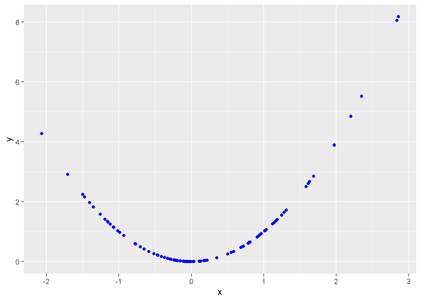
Figure 5.9: x and y are uncorrelated, but clearly related.

Chapter review

Over the course of this chapter and the previous one, we have learned the basic terminology and tools for working with random variables. These are the two most difficult chapters in the course, but if you work hard and develop your understanding of random variables you will find the rest of the course somewhat easier.

This is not a course on probability, so the next few chapters will be about data and statistics. We will first learn to use Excel to calculate common statistics from a cleaned data set. We will then use the tools of probability and random variables to build a theoretical framework in which we can interpret each statistic as a random variable and each data set as a collection of random variables. This theory will allow us to use statistics not only as a way of describing data, but as a way of understanding the process that produced that data.

Practice problems

Answers can be found in the appendix.

Questions 1- 7 below continue our craps example. To review that example, we have:

An outcome $(r,w)$ where $r$ and $w$ are the numbers rolled on a pair of fair six-sided dice
Several random variables defined in terms of that outcome:
- The total showing on the pair of dice: $t = r+w$
- An indicator for whether a bet on “Yo” wins: $y = I(t=11)$.

In addition, let $b = I(t=12)$ be an indicator of whether a bet on “Boxcars” wins. Since it is an indicator variable $b$ has the $Bernoulli(p)$ distribution with $p = 1/36$, so it has mean \[E(b) = p = 1/36\] and variance: \[var(b) = p(1-p) = 1/36*35/36 \approx 0.027 \]

SKILL #1: Derive a joint distribution from the underlying outcome

Let $f_{y,b}(\cdot)$ be the joint PDF of $y$ and $b$.
1. Find $f_{y,b}(1,1)$
2. Find $f_{y,b}(0,1)$
3. Find $f_{y,b}(1,0)$
4. Find $f_{y,b}(0,0)$

SKILL #2: Derive a marginal distribution from a joint distribution

Let $f_b(\cdot)$ be the marginal PDF of $b$
1. Find $f_b(0)$ based on the joint PDF $f_{y,b}(\cdot)$.
2. Find $f_b(1)$ based on the joint PDF $f_{y,b}(\cdot)$.
3. Find $E(b)$ based on this marginal PDF you found in parts (a) and (b).

SKILL #3: Derive a conditional distribution from a joint distribution

Let $f_{y|b}(1,1)$ be the conditional PDF of $y$ given $b$.
1. Find $f_{y|b}(1,1)$.
2. Find $f_{y|b}(0,1)$.
3. Find $f_{y|b}(1,0)$.
4. Find $f_{y|b}(0,0)$.

SKILL #4: Identify whether two random variables are independent

Which of the following pairs of random variables are independent?
- $y$ and $t$
- $y$ and $b$
- $r$ and $w$
- $r$ and $y$

SKILL #5: Find covariance from a PDF

Find $cov(y,b)$ using the joint PDF $f_{y,b}(\cdot)$.

SKILL #6: Find covariance using the alternate formula

Find the following covariances using the alternate formula:
1. Find $E(yb)$ using the joint PDF $f_{y,b}(\cdot)$.
2. Find $cov(y,b)$ using your result in (a).
3. Is your answer in (b) the same as your answer to question 5 above?

SKILL #7: Find correlation from covariance

Find $corr(y,b)$ using the results you found earlier.
We can find the correlation from the covariance, but we can also find the covariance from the correlation. For example, suppose we already know that \[\begin{align} E(t) &= 7 \\ var(t) &\approx 5.83 \\ corr(b,t) &\approx 0.35 \\ \end{align}\] Using this information and the values of $E(b)$ and $var(b)$ provided above:
1. Find $cov(b,t)$.
2. Find $E(bt)$.

SKILL #8: Find correlation and covariance for independent random variables

We earlier found that $r$ and $w$ were independent. Using this information:
1. Find $cov(r,w)$.
2. Find $corr(r,w)$.

SKILL #9: Work with linear functions of random variables

Your net winnings if you bet $1 on Yo and $1 on Boxcars can be written $16y + 31b - 2$. Find the following expected values:
1. Find $E(y + b)$
2. Find $E(16y + 31b - 2)$
Find the following variances and covariances:
1. Find $cov(16y,31b)$
2. Find $var(y + b)$

SKILL #10: Interpret covariances and correlations

Based on your results, which of the following statements is correct?
- The result of a bet on Boxcars is positively related to the result of a bet on Yo.
- The result of a bet on Boxcars is negatively related to the result of a bet on Yo.
- The result of a bet on Boxcars is not related to the result of a bet on Yo.

SKILL #11: Use the properties of the uniform distribution

Suppose that $x \sim U(-1,1)$.
1. Find the PDF $f_x(\cdot)$ of $x$
2. Find the CDF $F_x(\cdot)$ of $x$
3. Find $\Pr(x = 0)$
4. Find $\Pr(0 < x < 0.5)$
5. Find $\Pr(0 \leq x \leq 0.5)$
6. Find the median of $x$.
7. Find the 75th percentile of $x$.
8. Find $E(x)$
9. Find $var(x)$

SKILL #12: Work with linear functions of uniform random variables

Suppose that $x \sim U(-1,1)$, and let $y = 3x + 5$.
1. What is the probability distribution of $y$?
2. Find $E(y)$.

SKILL #13: Use the properties of the normal distribution

Suppose that $x \sim N(10,4)$.
1. Find $E(x)$.
2. Find the median of $x$.
3. Find $var(x)$.
4. Find $sd(x)$.
5. Use Excel to find $\Pr(x \leq 11)$.

SKILL #14: Work with linear functions of a normal random variable

Suppose that $x \sim N(10,4)$.
1. Find the distribution of $y = 3x + 5$.
2. Find a random variable $z$ that is a linear function of $x$ and has the standard normal distribution
3. Find an expression for $\Pr(x \leq 11)$ in terms of the standard normal CDF $\Phi(\cdot)$.
4. Use the Excel function NORM.S.DIST and the previous result to find to find the value of $\Pr(x \leq 11)$.

More precisely, either or both of $\sigma_x$ and $\sigma_y$ could be zero. In that case the covariance will also be zero, and the correlation will be undefined (zero divided by zero).↩︎