Simple Linear Regression
Setup
intall libraries
Explore relationships
Flow and area
m1<-lm(as.numeric(pp_area) ~ cur_in_mean, data = buf)

plot(buf$cur_mean, as.numeric(buf$pp_area), xlab="mean circuitscape current", ylab="pinch-point area")
abline(m1, col="red")
##
## Call:
## lm(formula = as.numeric(pp_area) ~ cur_in_mean, data = buf)
##
## Residuals:
##    Min     1Q Median     3Q    Max
## -55786 -14917 -13455  -7521 611100
##
## Coefficients:
##             Estimate Std. Error t value Pr(>|t|)
## (Intercept) 240277.0   124790.7   1.925   0.0548 .
## cur_in_mean  -1044.6      584.6  -1.787   0.0747 .
## ---
## Signif. codes:  0 '***' 0.001 '**' 0.01 '*' 0.05 '.' 0.1 ' ' 1
##
## Residual standard error: 54310 on 446 degrees of freedom
## Multiple R-squared:  0.007107,   Adjusted R-squared:  0.004881
## F-statistic: 3.192 on 1 and 446 DF,  p-value: 0.07466
Flow difference and area
m2<-lm(as.numeric(pp_area) ~ cur_diff, data = buf)

plot(buf$cur_diff, as.numeric(buf$pp_area), xlab="Difference between inner and outer current", ylab="pinch-point area")
abline(m2, col="red")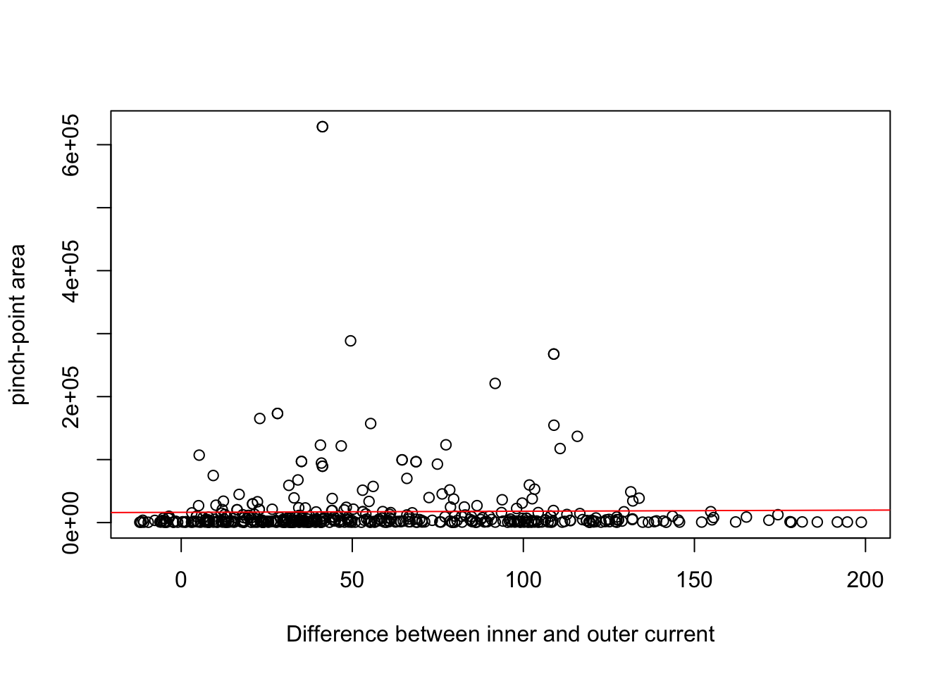
##
## Call:
## lm(formula = as.numeric(pp_area) ~ cur_diff, data = buf)
##
## Residuals:
##    Min     1Q Median     3Q    Max
## -19382 -15992 -14607  -8060 611518
##
## Coefficients:
##             Estimate Std. Error t value Pr(>|t|)
## (Intercept) 16313.83    4146.23   3.935 9.66e-05 ***
## cur_diff       18.22      56.91   0.320    0.749
## ---
## Signif. codes:  0 '***' 0.001 '**' 0.01 '*' 0.05 '.' 0.1 ' ' 1
##
## Residual standard error: 54500 on 446 degrees of freedom
## Multiple R-squared:  0.0002297,  Adjusted R-squared:  -0.002012
## F-statistic: 0.1025 on 1 and 446 DF,  p-value: 0.749
Flow and distance to city center
m4<-lm(as.numeric(dist2cent) ~ cur_in_mean, data = buf)

plot(buf$cur_mean, as.numeric(buf$dist2cent),  xlab="mean circuitscape current", ylab="distance to city center (m)")
abline(m4, col="red")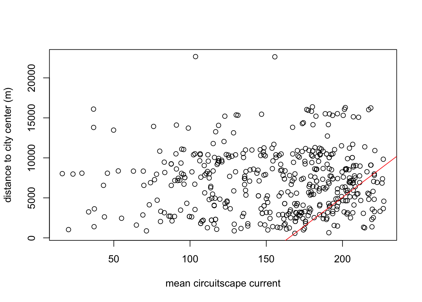
##
## Call:
## lm(formula = as.numeric(dist2cent) ~ cur_in_mean, data = buf)
##
## Residuals:
##     Min      1Q  Median      3Q     Max
## -6659.1 -3158.6    64.4  2605.5 15431.3
##
## Coefficients:
##              Estimate Std. Error t value Pr(>|t|)
## (Intercept) -23728.10    8874.54  -2.674 0.007777 **
## cur_in_mean    143.98      41.58   3.463 0.000586 ***
## ---
## Signif. codes:  0 '***' 0.001 '**' 0.01 '*' 0.05 '.' 0.1 ' ' 1
##
## Residual standard error: 3862 on 446 degrees of freedom
## Multiple R-squared:  0.02618,    Adjusted R-squared:  0.024
## F-statistic: 11.99 on 1 and 446 DF,  p-value: 0.000586
Flow difference and distance to city center
m5<-lm(as.numeric(dist2cent) ~ cur_diff, data = buf)

plot(buf$cur_diff, as.numeric(buf$dist2cent),  xlab="Difference between inner and outer current", ylab="distance to city center (m)")
abline(m5, col="red")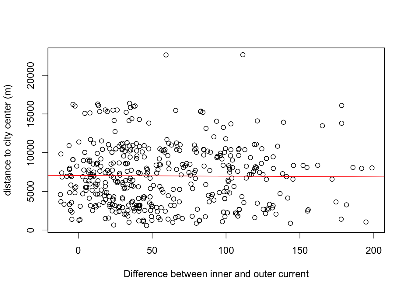
##
## Call:
## lm(formula = as.numeric(dist2cent) ~ cur_diff, data = buf)
##
## Residuals:
##    Min     1Q Median     3Q    Max
##  -6439  -3418    -14   2642  15708
##
## Coefficients:
##              Estimate Std. Error t value Pr(>|t|)
## (Intercept) 7046.0959   297.7544   23.66   <2e-16 ***
## cur_diff      -0.8588     4.0871   -0.21    0.834
## ---
## Signif. codes:  0 '***' 0.001 '**' 0.01 '*' 0.05 '.' 0.1 ' ' 1
##
## Residual standard error: 3914 on 446 degrees of freedom
## Multiple R-squared:  9.899e-05,  Adjusted R-squared:  -0.002143
## F-statistic: 0.04415 on 1 and 446 DF,  p-value: 0.8337
Flow difference and % vegetation cover (buffer)
m3<-lm(PRIMECLASS_VEG~cur_diff, data = buf)

plot(buf$cur_diff, buf$PRIMECLASS_VEG, xlab="Difference between inner and outer current", ylab="Proportion of vegetation cover")
abline(m3, col="red")
##
## Call:
## lm(formula = PRIMECLASS_VEG ~ cur_diff, data = buf)
##
## Residuals:
##      Min       1Q   Median       3Q      Max
## -0.61315 -0.09680  0.02327  0.11973  0.36589
##
## Coefficients:
##               Estimate Std. Error t value Pr(>|t|)
## (Intercept)  0.7883846  0.0134753   58.51   <2e-16 ***
## cur_diff    -0.0024433  0.0001852  -13.20   <2e-16 ***
## ---
## Signif. codes:  0 '***' 0.001 '**' 0.01 '*' 0.05 '.' 0.1 ' ' 1
##
## Residual standard error: 0.1765 on 441 degrees of freedom
##   (5 observations deleted due to missingness)
## Multiple R-squared:  0.2831, Adjusted R-squared:  0.2814
## F-statistic: 174.1 on 1 and 441 DF, p-value: < 2.2e-16m3b<-lm(PRIMECLASS_VEG~cur_diff, data = in_pp)
plot(in_pp$cur_diff, in_pp$PRIMECLASS_VEG, xlab="Difference between inner and outer current", ylab="Proportion of vegetation cover")
abline(m3b, col="red")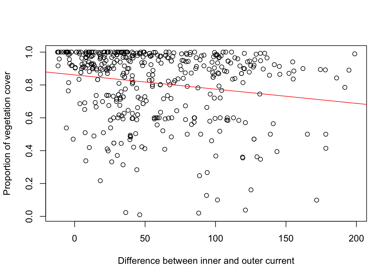
##
## Call:
## lm(formula = PRIMECLASS_VEG ~ cur_diff, data = in_pp)
##
## Residuals:
##     Min      1Q  Median      3Q     Max
## -0.8116 -0.1220  0.0807  0.1519  0.3006
##
## Coefficients:
##               Estimate Std. Error t value Pr(>|t|)
## (Intercept)  0.8612398  0.0160510  53.657  < 2e-16 ***
## cur_diff    -0.0008674  0.0002217  -3.912 0.000106 ***
## ---
## Signif. codes:  0 '***' 0.001 '**' 0.01 '*' 0.05 '.' 0.1 ' ' 1
##
## Residual standard error: 0.2091 on 436 degrees of freedom
##   (10 observations deleted due to missingness)
## Multiple R-squared:  0.03391,    Adjusted R-squared:  0.0317
## F-statistic: 15.31 on 1 and 436 DF,  p-value: 0.0001061
Flow difference and % developed (buffer)
m6<-lm(LANDCLAS_DEV~cur_diff, data = buf)

plot(buf$cur_diff, buf$LANDCLAS_DEV, xlab="Difference between inner and outer current", ylab="Proportion of developed land")
abline(m6, col="red")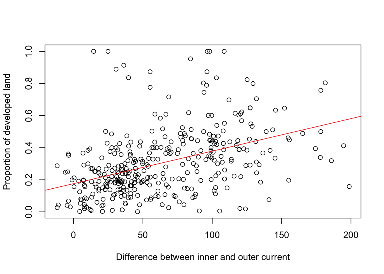
##
## Call:
## lm(formula = LANDCLAS_DEV ~ cur_diff, data = buf)
##
## Residuals:
##      Min       1Q   Median       3Q      Max
## -0.42097 -0.11945 -0.02463  0.08490  0.79492
##
## Coefficients:
##              Estimate Std. Error t value Pr(>|t|)
## (Intercept) 0.1756290  0.0169419  10.367   <2e-16 ***
## cur_diff    0.0020272  0.0002212   9.163   <2e-16 ***
## ---
## Signif. codes:  0 '***' 0.001 '**' 0.01 '*' 0.05 '.' 0.1 ' ' 1
##
## Residual standard error: 0.1867 on 377 degrees of freedom
##   (69 observations deleted due to missingness)
## Multiple R-squared:  0.1822, Adjusted R-squared:   0.18
## F-statistic: 83.97 on 1 and 377 DF,  p-value: < 2.2e-16
Flow difference and % developed (in pinch-point)
m7<-lm(LANDCLAS_DEV~cur_diff, data = in_pp)

plot(in_pp$cur_diff, in_pp$LANDCLAS_DEV, xlab="Difference between inner and outer current", ylab="Proportion of developed land")
abline(m7, col="red")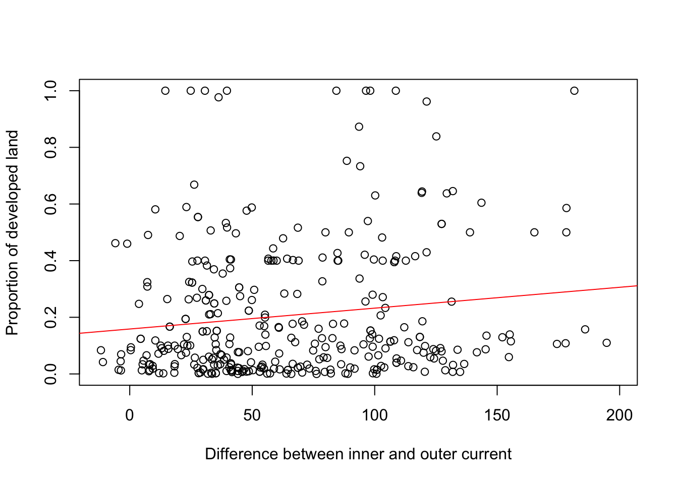
##
## Call:
## lm(formula = LANDCLAS_DEV ~ cur_diff, data = in_pp)
##
## Residuals:
##      Min       1Q   Median       3Q      Max
## -0.25088 -0.16902 -0.09455  0.13828  0.83064
##
## Coefficients:
##              Estimate Std. Error t value Pr(>|t|)
## (Intercept) 0.1586465  0.0229819   6.903 2.55e-11 ***
## cur_diff    0.0007374  0.0002952   2.498    0.013 *
## ---
## Signif. codes:  0 '***' 0.001 '**' 0.01 '*' 0.05 '.' 0.1 ' ' 1
##
## Residual standard error: 0.2331 on 336 degrees of freedom
##   (110 observations deleted due to missingness)
## Multiple R-squared:  0.01823,    Adjusted R-squared:  0.01531
## F-statistic: 6.239 on 1 and 336 DF,  p-value: 0.01297
4.0.1 Visualize for report
# set up regression plot function

custom_theme<-function(){theme(
        panel.background = element_rect(fill = "white",color="#636363"),
        axis.line.y = element_line(colour = "#636363"),
        axis.text.y = element_text(colour="#636363"),
        axis.ticks.y = element_line(colour = "#636363"),
        axis.title.y = element_text(colour="#636363"),
        axis.text.x = element_text(colour="#636363"),
        axis.ticks.x = element_line(colour = "#636363"),
        axis.line.x = element_line(colour = "#636363"),
        axis.title.x = element_text(colour="#636363"),
        legend.title = element_text(colour="#636363"),
        legend.text = element_text(colour="#636363"),
        legend.key = element_rect(fill = "white"),
      panel.grid.major = element_line(size = 0.0, colour="#bdbdbd")
)}


ggplotRegression <- function (fit) {

require(ggplot2)


ggplot(fit$model, aes_string(x = names(fit$model)[2], y = names(fit$model)[1])) +
  geom_point() +
  stat_smooth(method = "lm", col = "red") +
  labs(title = paste("Adj R2 = ",signif(summary(fit)$adj.r.squared, 5),
                     "Intercept =",signif(fit$coef[[1]],5 ),
                     " Slope =",signif(fit$coef[[2]], 5),
                     " P =",signif(summary(fit)$coef[2,4], 5)))+
         custom_theme()

}


fit1 <- lm(PRIMECLASS_VEG~cur_diff, data = buf)
fit2 <-lm(LANDCLAS_DEV~cur_diff, data = buf)
a<-ggplotRegression(fit1)
b<-ggplotRegression(fit2)
ggsave(filename = "4_output/regression/veg_curDif.png", a, height=5, width=8)
ggsave(filename = "4_output/regression/dev_curDif.png", b, height=5, width=8)