Circuitscape

Import the pinch-point and connectivity polygons derived from the circuitscape flow raster.

• check the crs
• visualize polygons
• clip to the study area (i.e. the North Saskatchewan Central region of the Ribbon of Green)

Import pinch-points

Load packages

library(sf)
library(tmap)
library(RColorBrewer)

Load spatial data

Load and plot the ribbon of green shape file RoG_Reaches_V1_210301.shp within the city boundary.

# load ribbon of green
RoG_Reaches<-st_read("1_data/external/Ribbon_of_Green_Study_Area_Reaches/Reach_Boundaries/RoG_Reaches_V1_210301/RoG_Reaches_V1_210301.shp")


# check crs
st_crs(RoG_Reaches)
# NAD83_3TM_114_Longitude_Meter_Province_of_Alberta_Canada
RoG_Reaches<-st_transform(RoG_Reaches, crs = st_crs(3776))

# load city boundary
City_Boundary<-st_read("1_data/external/City_Boundary/City_Boundary.shp")

# reproject to match the CRS of RoG_reaches 
City_Boundary<-st_transform(City_Boundary, crs = st_crs(3776))

#load road data
v_road<-st_read("1_data/external/roads_data/V_ROAD_SEGMENT_CUR.shp")
# reproject to match the CRS of RoG_reaches 
v_road<-st_transform(v_road, crs = st_crs(3776))

# crop roads file by a bounding box of the north saskatchewan central region polygon
v_road_1<-st_crop(v_road, City_Boundary)

#plot shape file
tmap_mode("plot")
m<-tm_shape(City_Boundary)+tm_borders(col = "#636363")+tm_fill(col="#d9d9d9")+
  tm_layout(frame=FALSE, legend.text.size=.5, legend.width=2, legend.position=c("left","bottom"),)+
  tm_legend(outside=TRUE, frame=FALSE)+
  tm_shape(v_road_1)+tm_lines(col="white", lwd = .8)+
  tm_shape(RoG_Reaches)+
   tm_fill(col="Reach", palette = "Paired", contrast = c(0.26, 1),alpha = .8, title="Ribbon of Green Reaches")+
   tm_borders(col = "#636363")
m



bbox_RoG<-st_bbox(RoG_Reaches)%>%
  st_as_sfc()

m<-
  tm_shape(bbox_RoG)+
    tm_borders(col="white")+
  tm_shape(City_Boundary)+
    tm_borders(col="#636363")+
    tm_fill(col="#d9d9d9")+
  tm_shape(v_road_1)+
    tm_lines(col="white", lwd = .8)+
  tm_shape(City_Boundary)+
    tm_borders(col="#636363")+
    tm_fill(col="#d9d9d9", alpha = 0)+
   # tm_legend(outside=TRUE, frame=FALSE)+ 
  tm_shape(RoG_Reaches)+
   tm_fill(col="Reach", palette = "Paired", contrast = c(0.26, 1),alpha = .8, title="Ribbon of Green Reaches")+
   tm_borders(col="#636363")+
  tm_layout(frame=FALSE, legend.text.size=.5, legend.outside = TRUE, legend.position = c("right", "top"))
m


tmap_save(m, "4_output/maps/ribbonGreen_map.png", outer.margins=c(0,0,0,0))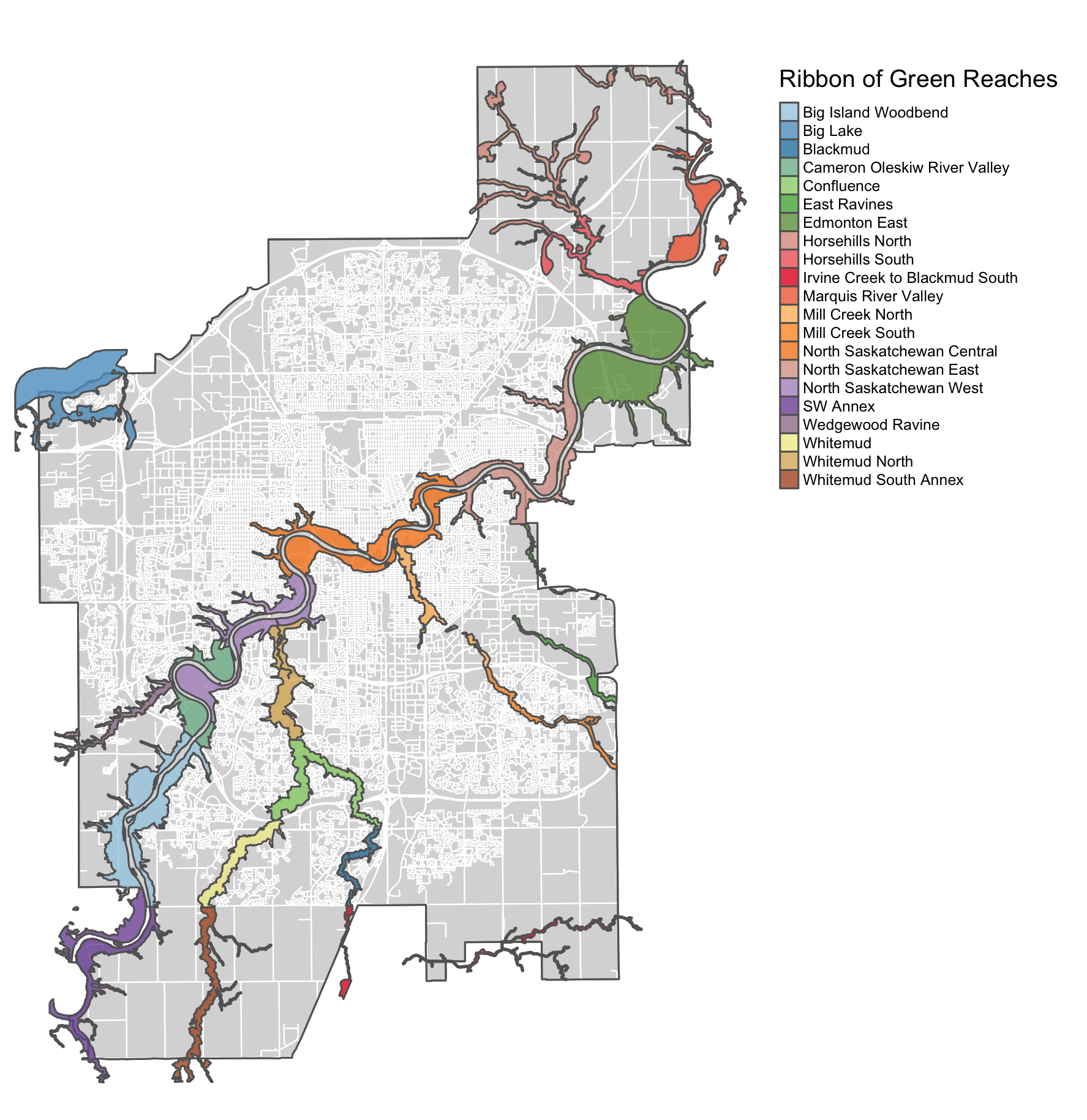

Figure 2.1: Ribbon of Green.

Define study area

For this project I focused on the North Central Region of Saskatchewan region of the ribbon of green

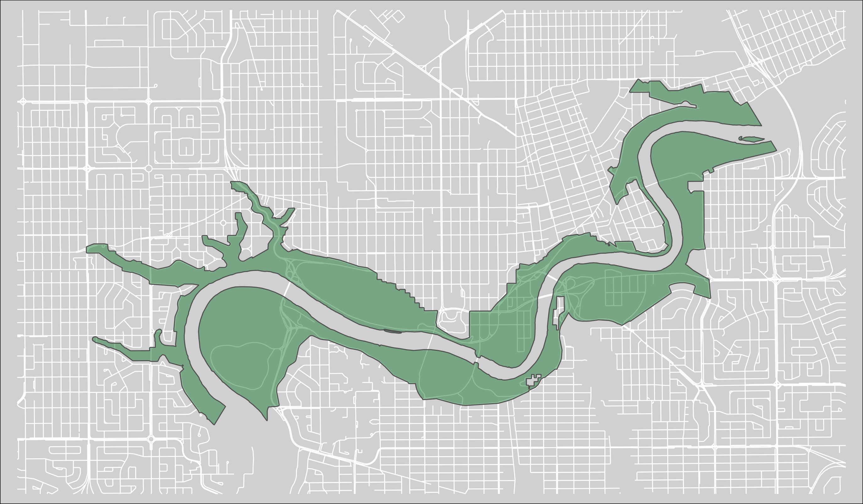
Figure 2.2: The North Saskatchewan Central region of the Ribbon of Green.

Load the connectivity and pinch-point polygons extracted from circuitscape

# Load summer coyote pinchpoints
pp_s<-st_read("1_data/external/Circuitscape/Data/PinchPoints/Data/Coyote_Summer_All_Pinchpoints.shp") %>% 
  st_buffer(dist=0)

# Load winter coyote pinchpoints
pp_w<-st_read("1_data/external/Circuitscape/Data/PinchPoints/Data/Coyote_Winter_All_Pinchpoints.shp") %>% 
  st_buffer(dist=0)

# load connetivity polygons
corridors<-st_read("1_data/external/Circuitscape/Vector_Extracted_Corridors/TerrestrialCorridor/TerrestrialCorridor.shp") %>% 
  st_buffer(dist=0)

corridors<-st_transform(corridors, crs = st_crs(3776))




#filter cooridors polygons to only include terrestrial connectivity polygons
#test<-corridors[corridors$ACoyotCor1=="0",]

---

Clip to study area

pp_s_clip<-st_intersection(pp_s, nscr)
#pp_s_clip<-st_intersection(pp_s, study_area)
pp_w_clip<-st_intersection(pp_w, nscr)
corridors_clip<-st_intersection(corridors, nscr)
#corridors_clip<-st_intersection(corridors, study_area)
save(pp_s_clip, file="1_data/manual/pp_s_clip.rData")
save(pp_w_clip, file="1_data/manual/pp_w_clip.rData")
save(corridors_clip, file="1_data/manual/corridors_clip.rData")

############# plot shape file #############################

# create a bounding box around study area
bbox<-st_bbox(nscr)
# crop roads file by a bounding box of the north saskatchewan central region polygon
v_road_3<-st_crop(v_road, bbox)


tmap_mode("plot")

m3<-
  tm_shape(v_road_3)+tm_lines(col="white")+
  tm_shape(nscr)+
    tm_fill(col="white", alpha=.6)+
    tm_borders(col = "#636363")+
  tm_shape(corridors_clip)+
   tm_fill(col="#238b45", alpha = .5)+
   tm_layout(bg.col="#d9d9d9")+
  tm_shape(pp_s_clip)+
    tm_fill(col="#fb6a4a", alpha = 1)+
    tm_borders(col = "#636363", lwd=1)+
  tm_layout(legend.outside = FALSE, legend.text.size = .9, legend.bg.color="white", legend.frame=TRUE, legend.frame.lwd=.8)+
    tm_add_legend(
      type="symbol", 
      shape=c(22,22, 22),
      col=c("#238b45", "#fb6a4a", "white"),
      alpha=c(.5, 1, 1),
      border.col = "black",
      border.lwd=.8,
      size=1.5,
      labels = c("movement corridors", "summer pinch-points", "N. Saskatchewan Central"))
m3

tmap_save(m3, "4_output/maps/pp_s_map.png", asp=0, outer.margins=c(0,0,0,0))


# library(OpenStreetMap)
# library(tmaptools)
# base<-read_osm(study_area, type="bing")
# 
# t<-st_buffer(corridors_clip,10)
# corridors_outline<-st_union(t)
# 
m3_b<-
  tm_shape(base) + tm_rgb()+
  tm_shape(study_area)+
    tm_fill(col="white", alpha=.2)+
  # tm_shape(v_road_clip)+tm_lines(col="white")+
  # tm_shape(nscr)+
  #   tm_fill(col="white", alpha=.6)+
  #   tm_borders(col = "#636363")+
  # tm_shape(corridors_clip)+
  #  tm_fill(col="#238b45", alpha = .5)+
  #  tm_layout(bg.col="#d9d9d9")+
  tm_shape(corridors_outline)+
  tm_fill(col="#238b45", alpha = .5)+
   tm_layout(bg.col="white")+
    tm_borders(col="#00441b", lwd=.7)+
  tm_shape(pp_s_clip)+
    tm_fill(col="#fb6a4a", alpha = 1)+
    tm_borders(col = "#fec44f", lwd=.5)+
  tm_layout(legend.outside = TRUE, legend.text.size = .9, legend.bg.color="white", legend.frame=TRUE, legend.frame.lwd=.8)+
    tm_add_legend(
      type="symbol",
      shape=c(22,22),
      col=c("#238b45", "#fb6a4a"),
      alpha=c(.5, 1),
      border.col = c("#00441b", "#fec44f"),
      border.lwd=.8,
      size=1.5,
      labels = c("movement corridors", "pinch-points"))
#m3_b

tmap_save(m3_b, "4_output/presentation/pp_s_map_b.png", asp=0, outer.margins=c(0,0,0,0))
# 
# 
# m3_b<-
#   tm_shape(base) + tm_rgb()+ 
#   tm_shape(study_area)+
#     tm_fill(col="white", alpha=.2)+
#   # tm_shape(v_road_clip)+tm_lines(col="white")+
#   # tm_shape(nscr)+
#   #   tm_fill(col="white", alpha=.6)+
#   #   tm_borders(col = "#636363")+
#   tm_shape(corridors_clip)+
#    tm_fill(col="#238b45", alpha = .5)+
#    tm_layout(bg.col="#d9d9d9")+
#   tm_shape(pp_s_clip)+
#     tm_fill(col="#fb6a4a", alpha = 1)+
#     tm_borders(col = "#636363", lwd=1)+
#   tm_layout(legend.outside = TRUE, legend.text.size = .9, legend.bg.color="white", legend.frame=TRUE, legend.frame.lwd=.8)+
#     tm_add_legend(
#       type="symbol", 
#       shape=c(22,22),
#       col=c("#238b45", "#fb6a4a"),
#       alpha=c(.5, 1),
#       border.col = "black",
#       border.lwd=.8,
#       size=1.5,
#       labels = c("movement corridors", "pinch-points"))
# m3_b
# 
# tmap_save(m3_b, "4_output/presentation/pp_s_map_b.png", asp=0, outer.margins=c(0,0,0,0))


m4<-
  tm_shape(v_road_3)+tm_lines(col="white")+
  tm_shape(nscr)+
  tm_fill(col="white", alpha=.6)+
    tm_borders(col = "#636363")+
  tm_shape(corridors_clip)+
   tm_fill(col="#238b45", alpha = .5)+
   tm_layout(bg.col="#d9d9d9")+
   tm_legend(outside= T)+
  tm_shape(pp_w_clip)+
    tm_fill(col="#3182bd", alpha = 1)+
    tm_borders(col = "#636363", lwd=.7)+
    tm_layout(legend.outside = FALSE, legend.text.size = .8, legend.bg.color="white", legend.frame=TRUE, legend.frame.lwd=1)+
    tm_add_legend(
      type="symbol", 
      shape=c(22,22, 22),
      col=c("#238b45", "#3182bd", "white"), 
      alpha=c(.5, 1, 1),
      border.col = "black",
      border.lwd=.8,
      size=1.5,
      labels = c("movement corridors", "winter pinch-points", "N. Saskatchewan Central"))
m4

tmap_save(m4, "4_output/maps/pp_w_map.png", asp=0, outer.margins=c(0,0,0,0))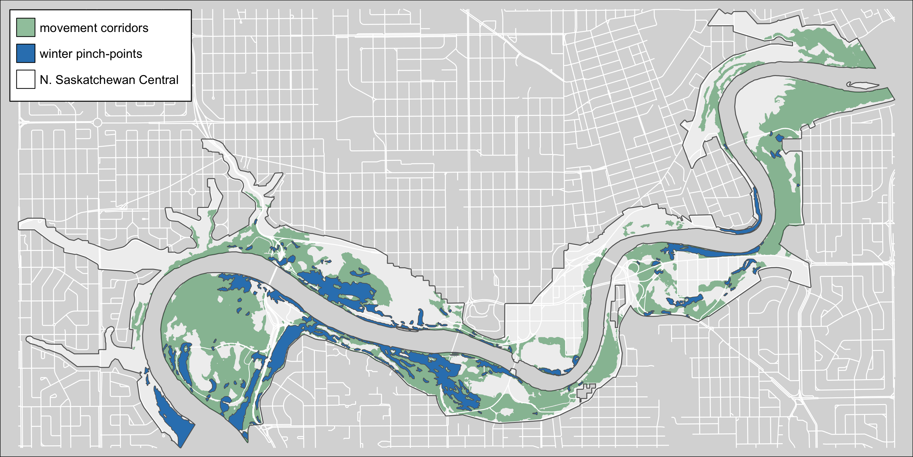

Figure 2.3: Winter terriestrical pinch-points within the North Saskatchewan Central region of the Ribbon of Green.

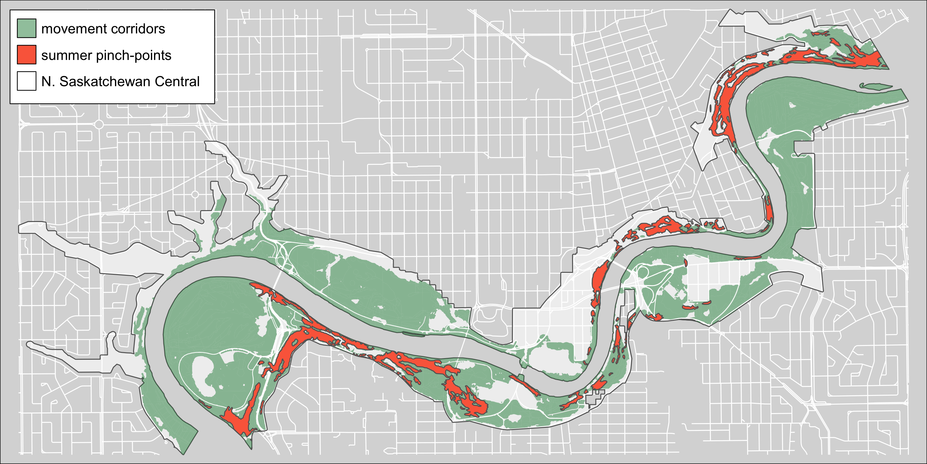
Figure 2.4: Summer terriestrical pinch-points within the North Saskatchewan Central region of the Ribbon of Green.

---

Cluster pinch-points

There are groups of pinch points very close to each other. This will lead to significant overlap in buffers. Since neighboring pinch-points will likely be caused by similar biophysical features, I decided to group neighboring pinch-points. Below, polygons are clustered based on a user defined threshold. I chose a 50 m threshold.

Filter out small pinch-point polygons

# x<-pp_s_clip

#calculate the are of each polygon
x$area <- st_area(x)

# filter out polygons based on minimum area
## set min area (m^2)
m<-5000

library(units) #use this package to convert the threshold value to a units object
m=set_units(m, m^2)
f<-x$area>m
x_f=x[f,]

Cluster remaining polygons by proximity

# here is a function that takes an SF object, clusters features within a specified distance threshold, and merges them into a new object

clusterSF <- function(sfpolys, thresh){
    dmat = st_distance(sfpolys)
    hc = hclust(as.dist(dmat>thresh), method="single")
    groups = cutree(hc, h=0.5)
    d = st_sf(
        geom = do.call(c,
            lapply(1:max(groups), function(g){
                st_union(sfpolys[groups==g,])
            })
            )
        )
    d$group = 1:nrow(d)
    d
}

#set a distance threshold to group polygons
t<-25


pp_s_clip_clus<-clusterSF(x_f, set_units(t, m))

save(pp_s_clip_clus, file="3_pipeline/tmp/pp_s_clip_clus.rData")




## plot clustered pinch-points
tmap_mode("plot")

m5<-
  tm_shape(v_road_3)+tm_lines(col="white")+
  tm_layout(bg.col="#d9d9d9")+
  tm_shape(nscr)+
    tm_fill(col="white", alpha=.4)+
    tm_borders(col = "#636363")+
  tm_shape(pp_s_clip_clus)+
    tm_fill(col="MAP_COLORS", palette = "Dark2", contrast = c(0.26, 1),alpha = 1, n= nrow(pp_s_clip_clus), legend.show = FALSE)+
  tm_borders(col = "#636363")
m5

tmap_save(m5, "4_output/maps/pp_s_clus_map.png", asp=0, outer.margins=c(0,0,0,0))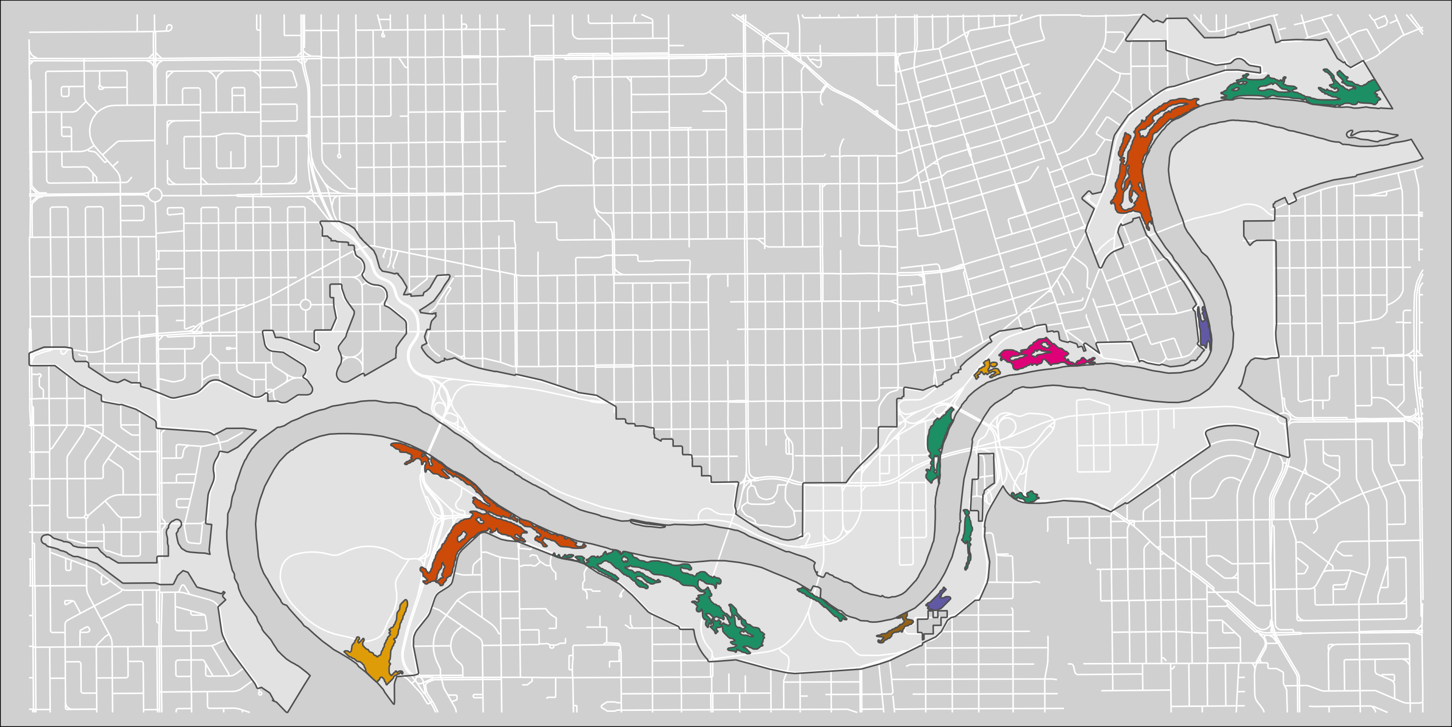

Figure 2.5: Clusters of pinch-points within 50m of each other.

---

Buffer pinch-points

Create an exterior buffer around pinch-point polygons. We will later characterize features within these buffers. I used a 30 m buffer.

pp_s_clip_clus_buf<-st_buffer(pp_s_clip_clus, dist= 30, singleSide = TRUE,  endCapStyle = "ROUND",
  joinStyle = "ROUND")

save(pp_s_clip_clus_buf, file="3_pipeline/store/pp_s_clip_clus_buf.rData")

## plot buffered clusters

m6<-
  tm_shape(v_road_3)+tm_lines(col="white")+
  tm_layout(bg.col="#d9d9d9")+
  tm_shape(nscr)+
    tm_fill(col="white", alpha=.4)+
    tm_borders(col = "#636363")+
  tm_shape(pp_s_clip_clus_buf)+
    tm_fill(col="MAP_COLORS", palette = "Dark2", contrast = c(0.26, 1),alpha = 1, n= nrow(pp_s_clip_clus), legend.show = FALSE)+
  tm_borders(col = "#636363")
m6

tmap_save(m6, "4_output/maps/pp_s_clus_buf_map.png", asp=0, outer.margins=c(0,0,0,0))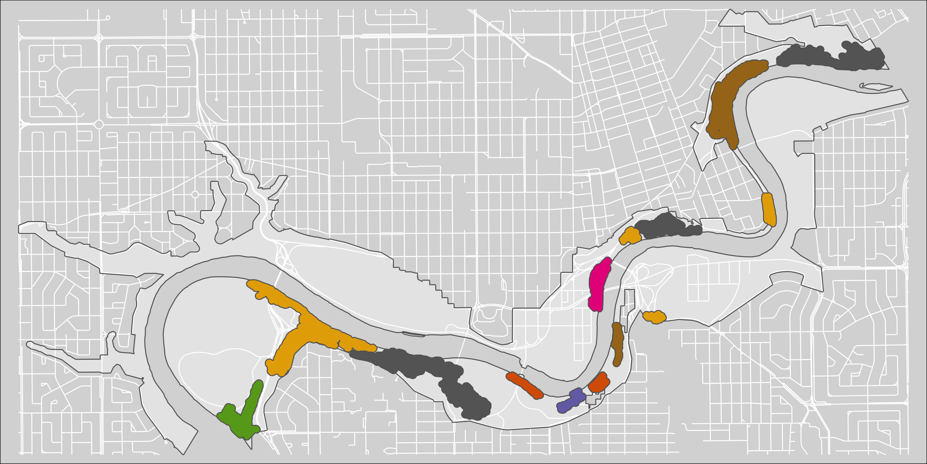

Figure 2.6: Clusters of pinch-points with a 30m buffer.

Exterior only buffer

pp_s_clip_clus_buf_ext<-st_buffer(st_boundary(pp_s_clip_clus), dist= 30, singleSide = TRUE,  endCapStyle = "ROUND",
  joinStyle = "ROUND")

#create a unique ID column
pp_s_clip_clus_buf_ext<-cbind(ID=1:nrow(pp_s_clip_clus_buf_ext), pp_s_clip_clus_buf_ext)
save(pp_s_clip_clus_buf_ext, file="3_pipeline/store/pp_s_clip_clus_buf_ext.rData")

## plot buffered clusters

m7<-
  tm_shape(v_road_3)+tm_lines(col="white")+
  tm_layout(bg.col="#d9d9d9")+
  tm_shape(nscr)+
    tm_fill(col="white", alpha=.4)+
    tm_borders(col = "#636363")+
  tm_shape(pp_s_clip_clus_buf_ext)+
    tm_fill(col="MAP_COLORS", palette = "Dark2", contrast = c(0.26, 1),alpha = 1, n= nrow(pp_s_clip_clus), legend.show = FALSE)+
  tm_borders(col = "#636363")
m7

tmap_save(m7, "4_output/maps/pp_s_clus_buf_ext_map.png", asp=0, outer.margins=c(0,0,0,0))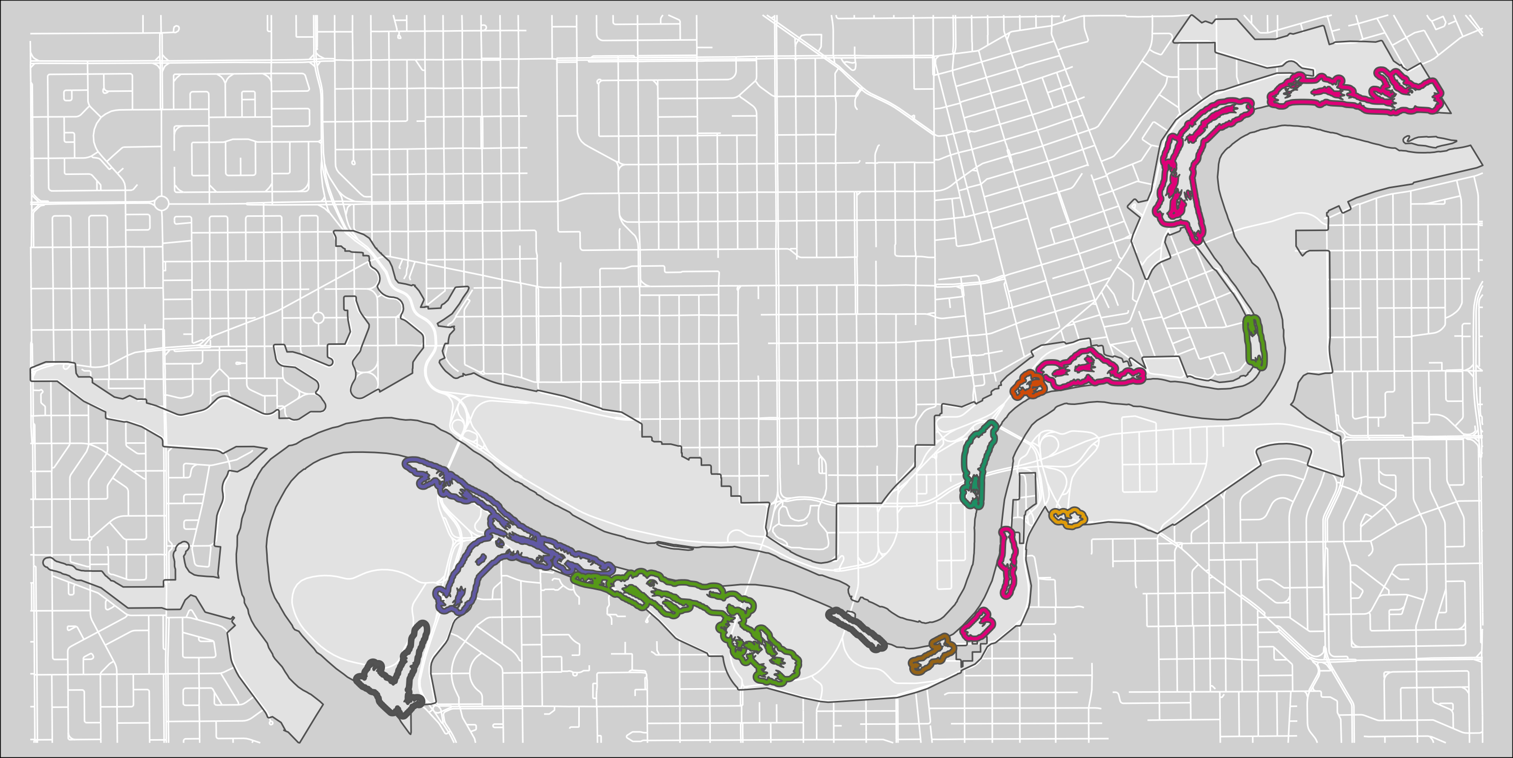

Figure 2.7: Clusters of pinch-points with a 30m exterior buffer.

---

Current map

Load and clip the terrestrial circuitscape current map.

Summer coyote

cur_map_sum<-raster("1_data/external/Circuitscape/Map/Coyote_Summer_All_curmap.tif")

projectRaster(cur_map_sum, crs=st_crs(study_area))

cur_map_sum_clip<-crop(cur_map_sum, study_area)

save(cur_map_sum_clip, file="1_data/manual/cur_map_sum_clip.rData")

m8<-
  tm_shape(cur_map_sum_clip)+
    tm_raster(palette="-RdBu",
              title = "Current",
              style="cont",
              drop.levels = TRUE,
              contrast = c(0,1)
              )+
  tm_layout(legend.show = FALSE,
            legend.outside = FALSE, 
            legend.text.size = .8, 
            legend.bg.color="white", 
            legend.frame=TRUE,
            legend.title.size=1, 
            legend.frame.lwd=.8,
            )
m8

tmap_save(m8, "4_output/maps/cur_map_sum_map.png", outer.margins=c(0,0,0,0))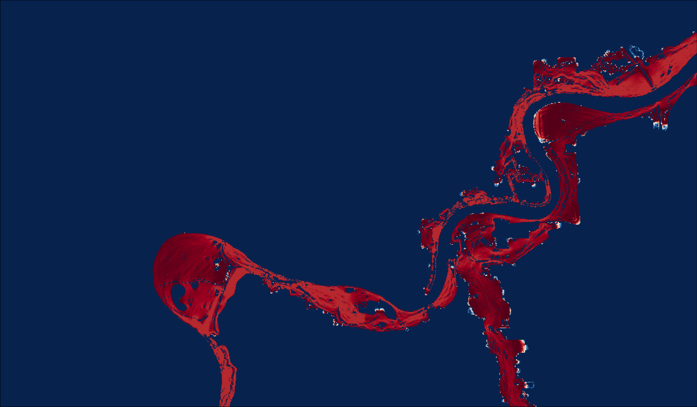 

Figure 2.8: Summer coyote current map.

Winter coyote

cur_map_win<-raster("1_data/external/Circuitscape/Map/Coyote_Winter_All_curmap.tif")

projectRaster(cur_map_win, crs=crs(study_area))

cur_map_win_clip<-crop(cur_map_win, study_area)

save(cur_map_win_clip, file="1_data/manual/cur_map_win_clip.rData")


m9<-
  tm_shape(cur_map_win_clip)+
    tm_raster(palette="-RdBu",
              title = "Current",
              style="cont",
              contrast = c(0,1),
              )+
  tm_layout(legend.show = FALSE,
            legend.outside = FALSE, 
            legend.text.size = .8, 
            legend.bg.color="white", 
            legend.frame=TRUE,
            legend.title.size=1, 
            legend.frame.lwd=.8,
            )
m9

tmap_save(m9, "4_output/maps/cur_map_win_map.png", outer.margins=c(0,0,0,0))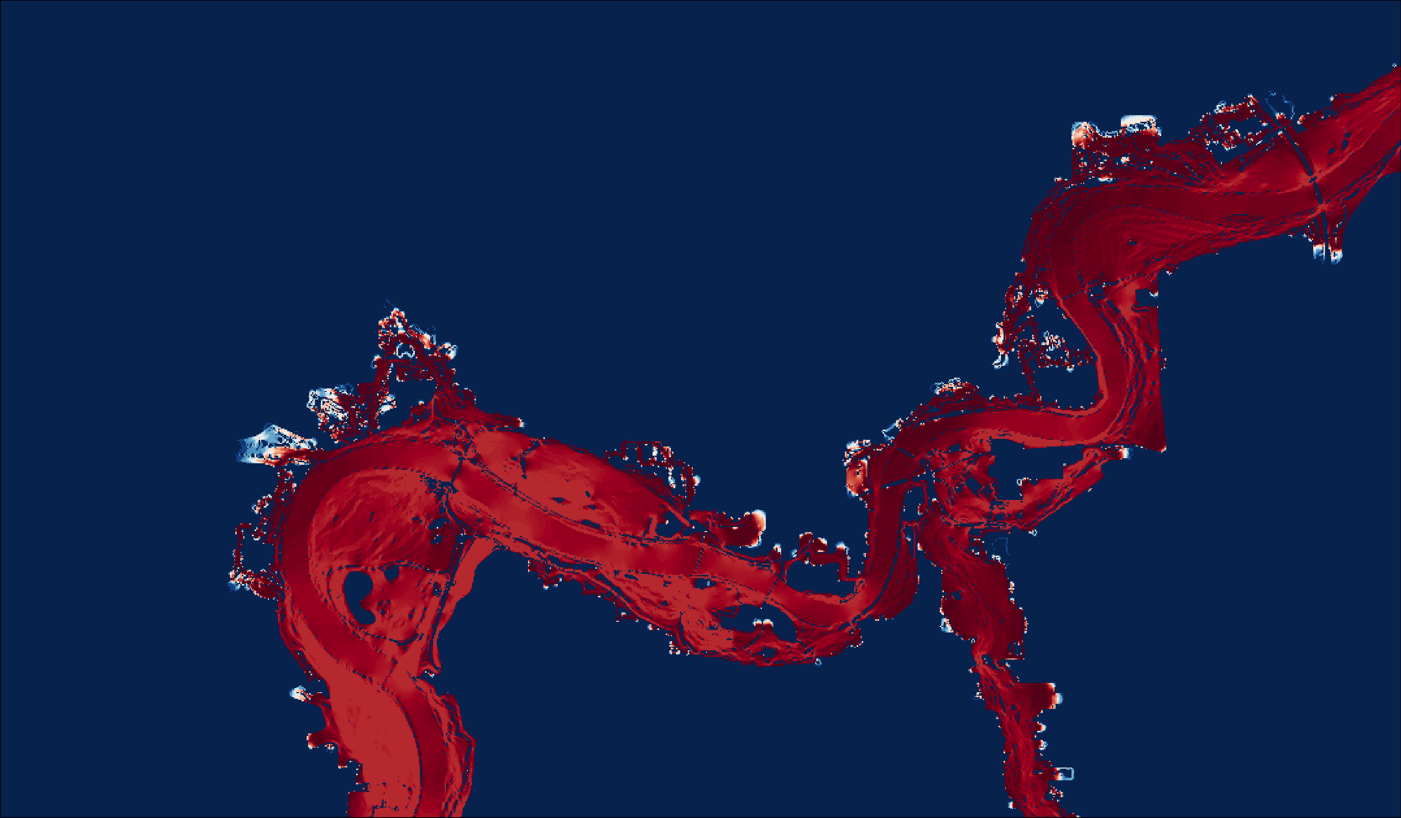 

Figure 2.9: Winter coyote current map.