PCA (pinch-point buffers)
Setup
intall libraries
Run PCA
Prep data and run PCA
x<-pp_all_Met_wide
x<-x[-c(1)]
x<-distinct(x)

rownames(x)<-x[,1]
x<-x[-c(1)]

x$pp_area<-as.numeric(x$pp_area)
x$pp_area<-as.numeric(x$dist2cent)

x[is.na(x)]<-0

#create grouping variable
x$area_group <- cut(x$pp_area, 4)

# x.pca<-prcomp(x[,c(8, 11:27)], center = TRUE, scale. = TRUE)
# summary(x.pca)

x.pca<-princomp(x[,c(12:28)], cor=TRUE)
summary(x.pca)
print(x.pca$loadings)
save(x.pca, file="3_pipeline/tmp/x.pca_out.rData")

x.pca$scores

#save output as a txt file
sink("4_output/PCA/summary_pca.txt")
print(summary(x.pca))
sink()

# x.pca_2<-princomp(x[,c(8:9, 11:57)], cor=TRUE)
# summary(x.pca_2)

x.pca<-princomp(x[,c(4:5, 8:9, 11:27)], cor=TRUE)
# summary(x.pca_2)
##
## Loadings:
## Comp.1 Comp.2 Comp.3 Comp.4 Comp.5 Comp.6 Comp.7 Comp.8 Comp.9
## trail_proportion 0.143 0.263 0.254 0.253 0.443 0.103 0.457
## trail_tot_buf 0.509 -0.178 0.182 0.182 0.238 0.314
## road_proportion 0.177 0.429 0.166 -0.402 -0.571 0.142
## road_tot_buf 0.568 -0.195 -0.134 -0.220 -0.109
## canopy_grass -0.196 -0.261 0.206 0.161 0.431 0.296
## canopy_shrub_con 0.445 -0.202 -0.246 -0.477
## canopy_shrub_dec 0.144 0.144 0.187 -0.247 0.103 -0.429 0.300 0.435 -0.520
## canopy_tree_con 0.391 0.201 0.252
## canopy_tree_dec 0.395 0.216 0.235
## PRIMECLASS_NVE -0.316 0.469
## PRIMECLASS_VEG 0.317 -0.468
## LANDCLAS_DEV -0.359 0.252 0.239 -0.267 -0.156 0.190 0.131 0.200
## LANDCLAS_MOD -0.247 -0.453 0.107 0.118 -0.342
## LANDCLAS_NAT 0.314 -0.325 0.481 0.327 -0.234 -0.204 -0.264
## LANDCLAS_NAW 0.403 0.193 -0.291 0.112
## LANDCLAS_NNW 0.208 -0.370 0.304 -0.466 0.534
## LANDCLAS_WET -0.141 -0.367 -0.323 0.182 -0.615 0.453
## Comp.10 Comp.11 Comp.12 Comp.13 Comp.14 Comp.15 Comp.16
## trail_proportion 0.465 0.185 0.321
## trail_tot_buf -0.474 0.127 0.197 -0.448
## road_proportion 0.453 -0.142
## road_tot_buf -0.282 -0.331 0.599
## canopy_grass -0.609 -0.369 -0.169
## canopy_shrub_con 0.617 0.129 -0.263
## canopy_shrub_dec 0.147 -0.260 -0.119 -0.124
## canopy_tree_con 0.208 -0.396 -0.271 0.673
## canopy_tree_dec 0.144 -0.346 -0.206 -0.733
## PRIMECLASS_NVE 0.514
## PRIMECLASS_VEG 0.649 -0.495
## LANDCLAS_DEV 0.104 -0.135 0.349
## LANDCLAS_MOD 0.387 -0.190 -0.148 0.240 0.561
## LANDCLAS_NAT -0.128 0.128 0.237
## LANDCLAS_NAW -0.478 0.243 0.248 0.580
## LANDCLAS_NNW 0.145 0.226 0.173 0.132 0.308
## LANDCLAS_WET 0.136 -0.253 -0.153
## Comp.17
## trail_proportion
## trail_tot_buf
## road_proportion
## road_tot_buf
## canopy_grass
## canopy_shrub_con
## canopy_shrub_dec
## canopy_tree_con
## canopy_tree_dec
## PRIMECLASS_NVE 0.633
## PRIMECLASS_VEG
## LANDCLAS_DEV -0.636
## LANDCLAS_MOD
## LANDCLAS_NAT -0.436
## LANDCLAS_NAW
## LANDCLAS_NNW
## LANDCLAS_WET
##
## Comp.1 Comp.2 Comp.3 Comp.4 Comp.5 Comp.6 Comp.7 Comp.8 Comp.9
## SS loadings 1.000 1.000 1.000 1.000 1.000 1.000 1.000 1.000 1.000
## Proportion Var 0.059 0.059 0.059 0.059 0.059 0.059 0.059 0.059 0.059
## Cumulative Var 0.059 0.118 0.176 0.235 0.294 0.353 0.412 0.471 0.529
## Comp.10 Comp.11 Comp.12 Comp.13 Comp.14 Comp.15 Comp.16 Comp.17
## SS loadings 1.000 1.000 1.000 1.000 1.000 1.000 1.000 1.000
## Proportion Var 0.059 0.059 0.059 0.059 0.059 0.059 0.059 0.059
## Cumulative Var 0.588 0.647 0.706 0.765 0.824 0.882 0.941 1.000## Importance of components:
## Comp.1 Comp.2 Comp.3 Comp.4 Comp.5
## Standard deviation 2.0501756 1.6063640 1.4153011 1.23455676 1.13107646
## Proportion of Variance 0.2472482 0.1517885 0.1178281 0.08965473 0.07525494
## Cumulative Proportion 0.2472482 0.3990368 0.5168648 0.60651958 0.68177452
## Comp.6 Comp.7 Comp.8 Comp.9 Comp.10
## Standard deviation 1.05932611 0.97054331 0.92307307 0.80745759 0.77885008
## Proportion of Variance 0.06601011 0.05540908 0.05012141 0.03835222 0.03568279
## Cumulative Proportion 0.74778462 0.80319370 0.85331511 0.89166733 0.92735012
## Comp.11 Comp.12 Comp.13 Comp.14
## Standard deviation 0.68884070 0.57698413 0.57216093 0.315966626
## Proportion of Variance 0.02791185 0.01958298 0.01925695 0.005872642
## Cumulative Proportion 0.95526197 0.97484495 0.99410190 0.999974543
## Comp.15 Comp.16 Comp.17
## Standard deviation 2.080303e-02 2.275737e-08 0
## Proportion of Variance 2.545683e-05 3.046458e-17 0
## Cumulative Proportion 1.000000e+00 1.000000e+00 1Visualize eigenvalues (scree plot).
How much variance is explained by each principal componant?
png("4_output/PCA/scree_plot", width=1000, height=600)
fviz_eig(x.pca)
dev.off()

# Contributions of variables to PC1
png("4_output/PCA/cont_PCA1_plot", width=1000, height=600)
fviz_contrib(x.pca, choice = "var", axes = 1, top = 10)
dev.off()


# Contributions of variables to PC2
png("4_output/PCA/cont_PCA2_plot", width=1000, height=600)
fviz_contrib(x.pca, choice = "var", axes = 2, top = 10)
dev.off()
Figure 4.1: Scree plot showing how much variance is explained by each PCA
Figure 4.2: Contribution of variables to Dim-1
Figure 4.3: Contribution of variables to Dim-2
Plot results
# create ggplot theme
custom_theme<-function(){theme(
        panel.background = element_rect(fill = "white", color="#636363"),
        # axis.line.y = element_line(colour = "#636363"),
        axis.text.y = element_text(colour="#636363"),
        axis.ticks.y = element_line(colour = "#636363"),
        axis.title.y = element_text(colour="#636363"),
        axis.text.x = element_text(colour="#636363"),
        axis.ticks.x = element_line(colour = "#636363"),
        #axis.line.x = element_line(colour = "#636363"),
        axis.title.x = element_text(colour="#636363"),
        legend.title = element_text(colour="#636363"),
        legend.text = element_text(colour="#636363"),
        legend.key = element_rect(fill = "white"),
      panel.grid.major = element_line(size = 0.0, colour="#bdbdbd"),
      aspect.ratio = 5/5
        #panel.grid.minor = element_line(size = 0.0)
        )}


# with labels
ggbiplot(x.pca, circle = TRUE)+
  custom_theme()
ggsave(filename="4_output/PCA/pca.png",  width = 13, height = 10)


#current difference
ggbiplot(x.pca,  ellipse=TRUE, groups=x$cur_diff_group)+
  labs(color="current difference")+
    custom_theme()
ggsave(filename="4_output/PCA/pca_cur_diff_group.png",  width = 13, height = 10)


#mean current
ggbiplot(x.pca,  ellipse=TRUE, groups=x$cur_in_mean_group)+
  labs(color="Mean current in pinch-point")+
    custom_theme()
ggsave(filename="4_output/PCA/pca_cur_in_mean_group.png", width = 13, height = 10)


#distance 2 city center
ggbiplot(x.pca,  ellipse=TRUE, groups=x$dist2cent_group)+
  labs(color="distance to city center")+
    custom_theme()
ggsave(filename="4_output/PCA/pca_dist2cent_group.png", width = 13, height = 10)


#reach
ggbiplot(x.pca,  ellipse=TRUE, groups=x$Reach)+
  labs(color="RoG reach")+
    custom_theme()
ggsave(filename="4_output/PCA/pca_Reach_group.png", width = 13, height = 10)


#polygon area
ggbiplot(x.pca,  ellipse=TRUE, groups=x$area_group)+
  labs(color="pinch-point area (m)")+
    custom_theme()
ggsave(filename="4_output/PCA/pca_area_group.png", width = 13, height = 10)


#polygon area
ggbiplot(x.pca,  ellipse=TRUE, groups=x$season)+
  labs(color="season")+
    custom_theme()
ggsave(filename="4_output/PCA/pca_season_group.png", width = 13, height = 10)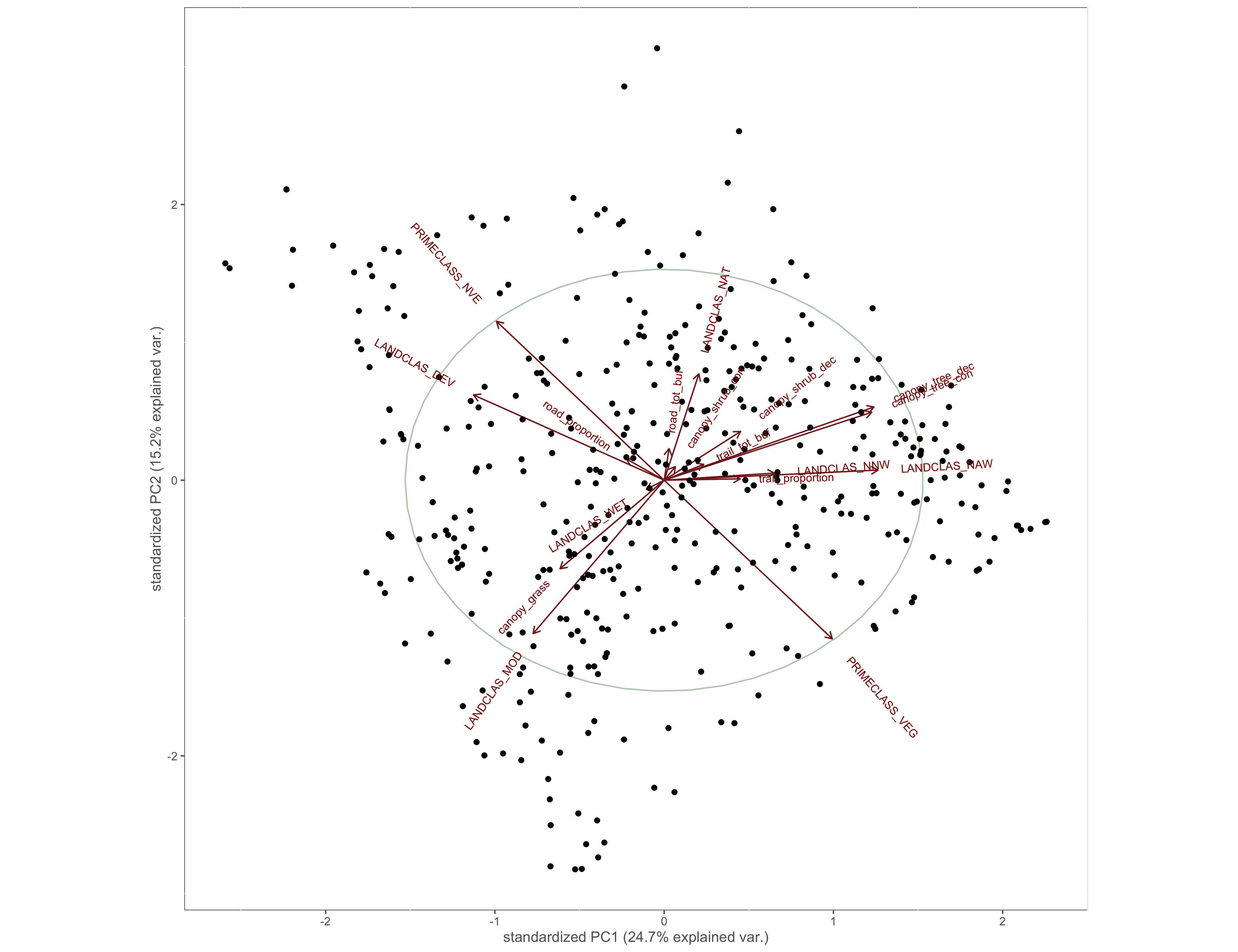
Figure 4.4: PCA results
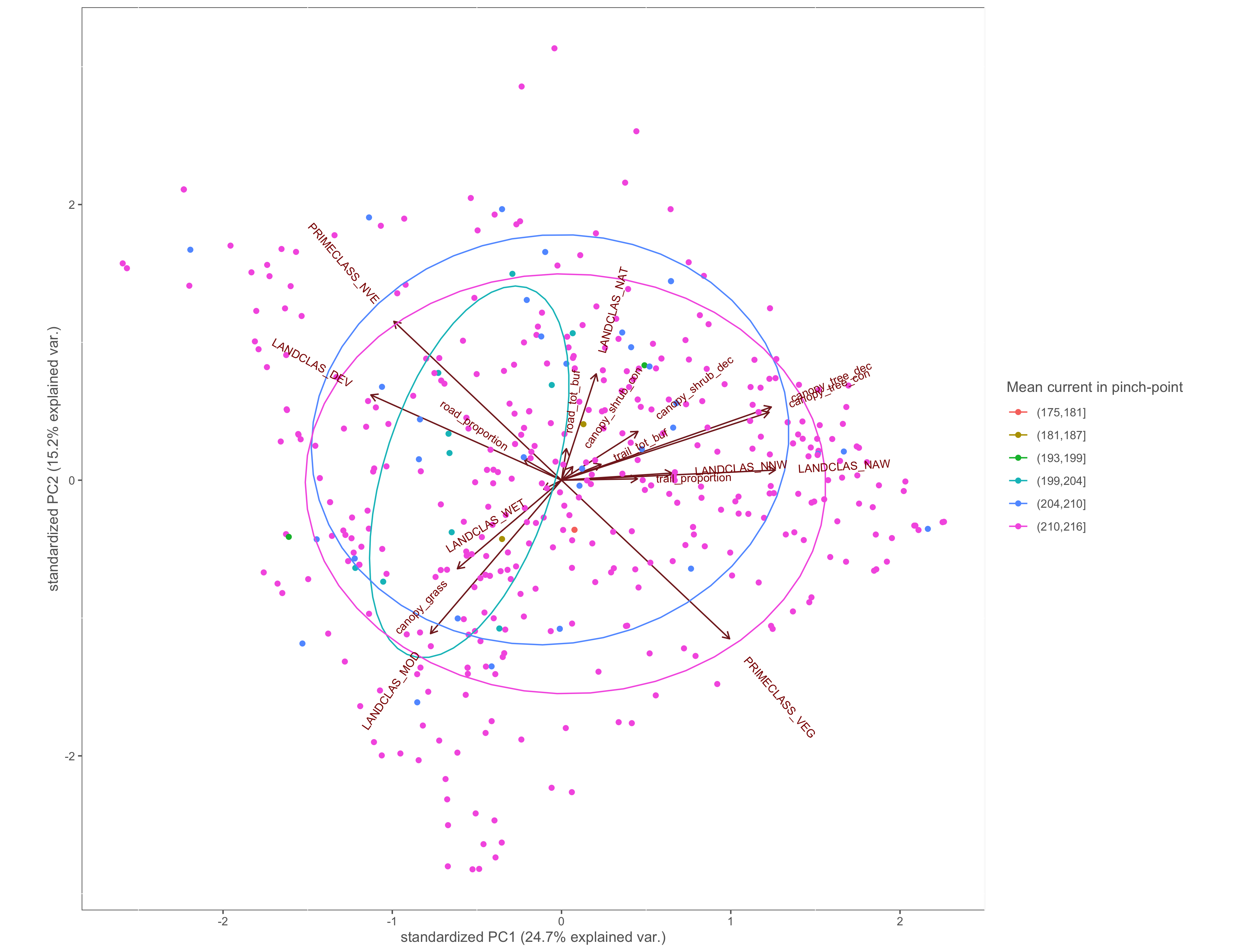
Figure 4.5: PCA biplot with pinch-points grouped by the within pinch-pont mean current values
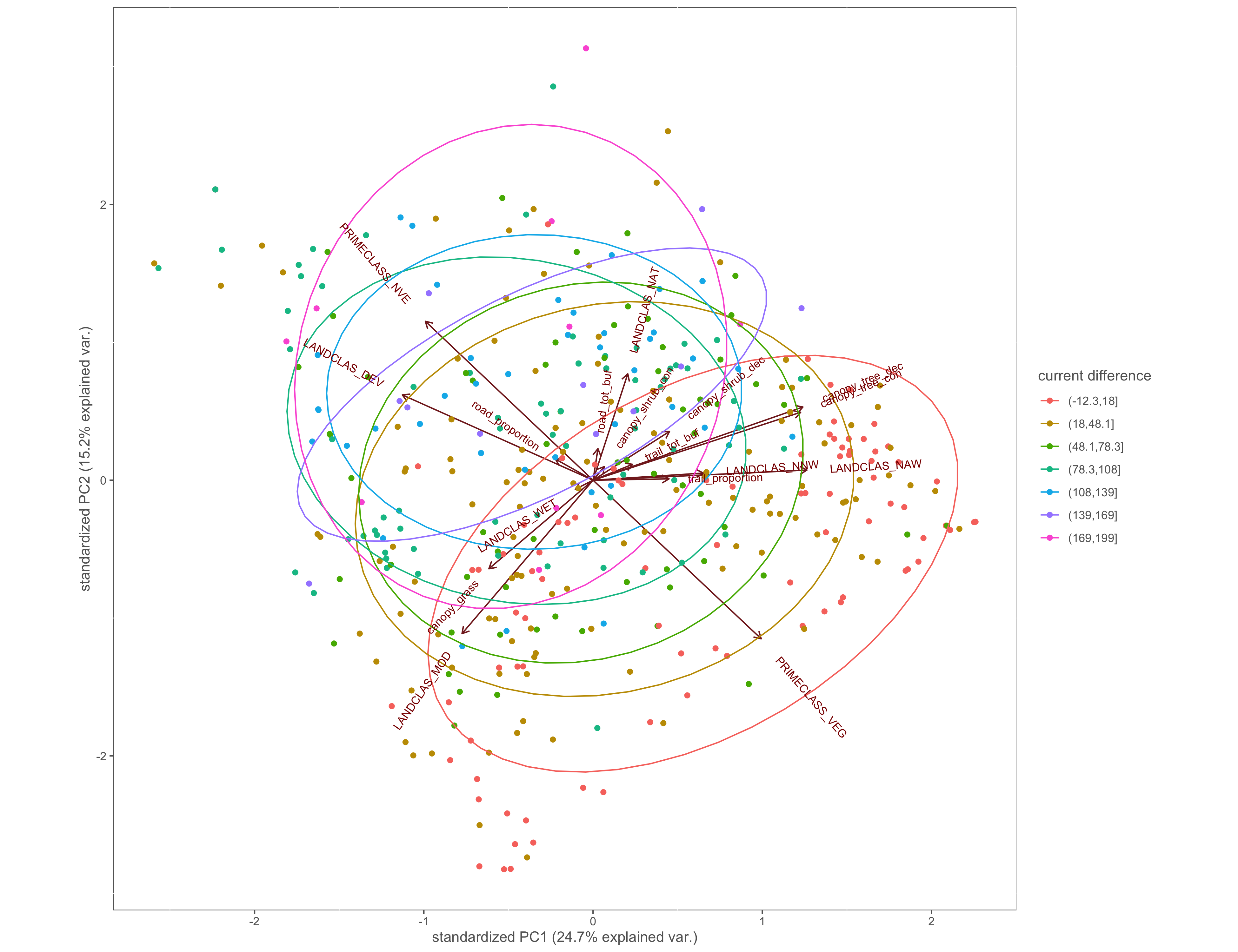
Figure 4.6: PCA biplot with pinch-points grouped by the difference between within and without current values
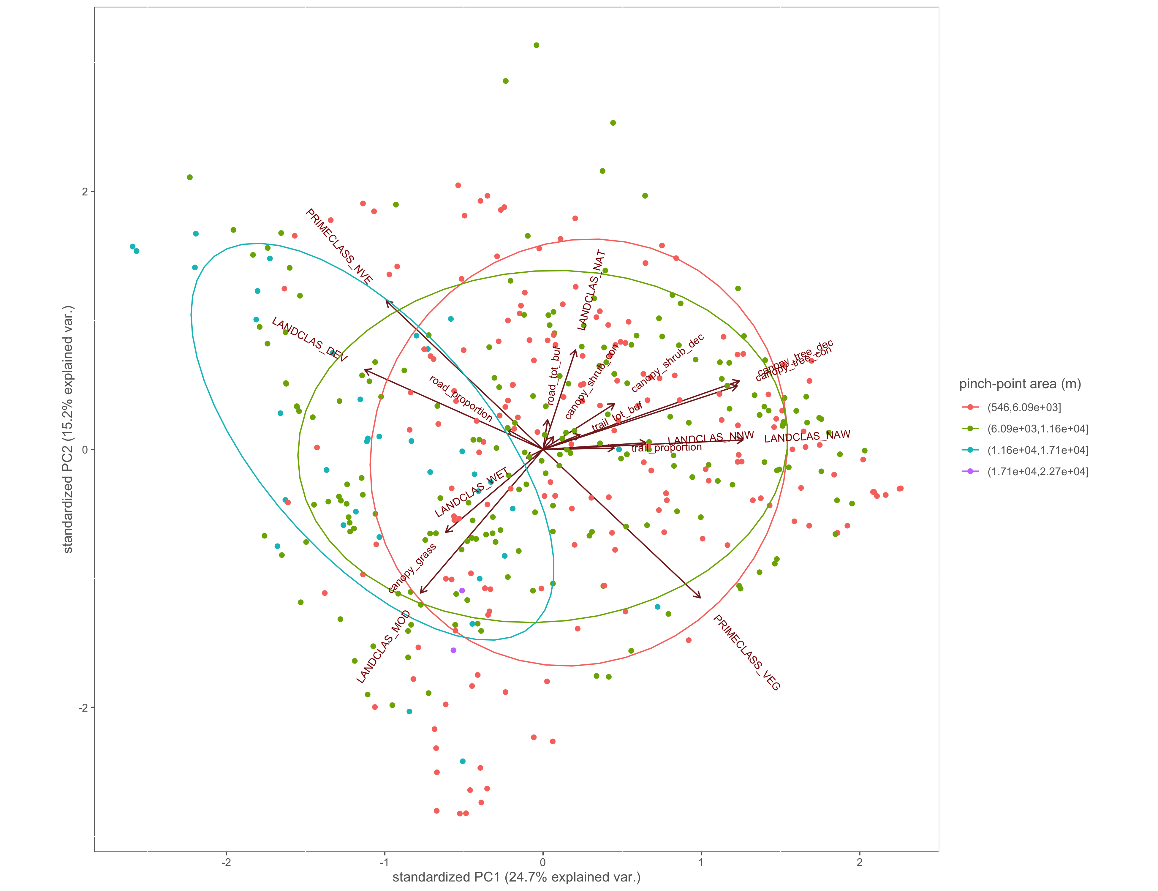
Figure 4.7: PCA biplot with pinch-points grouped by the pinch-point polygon area
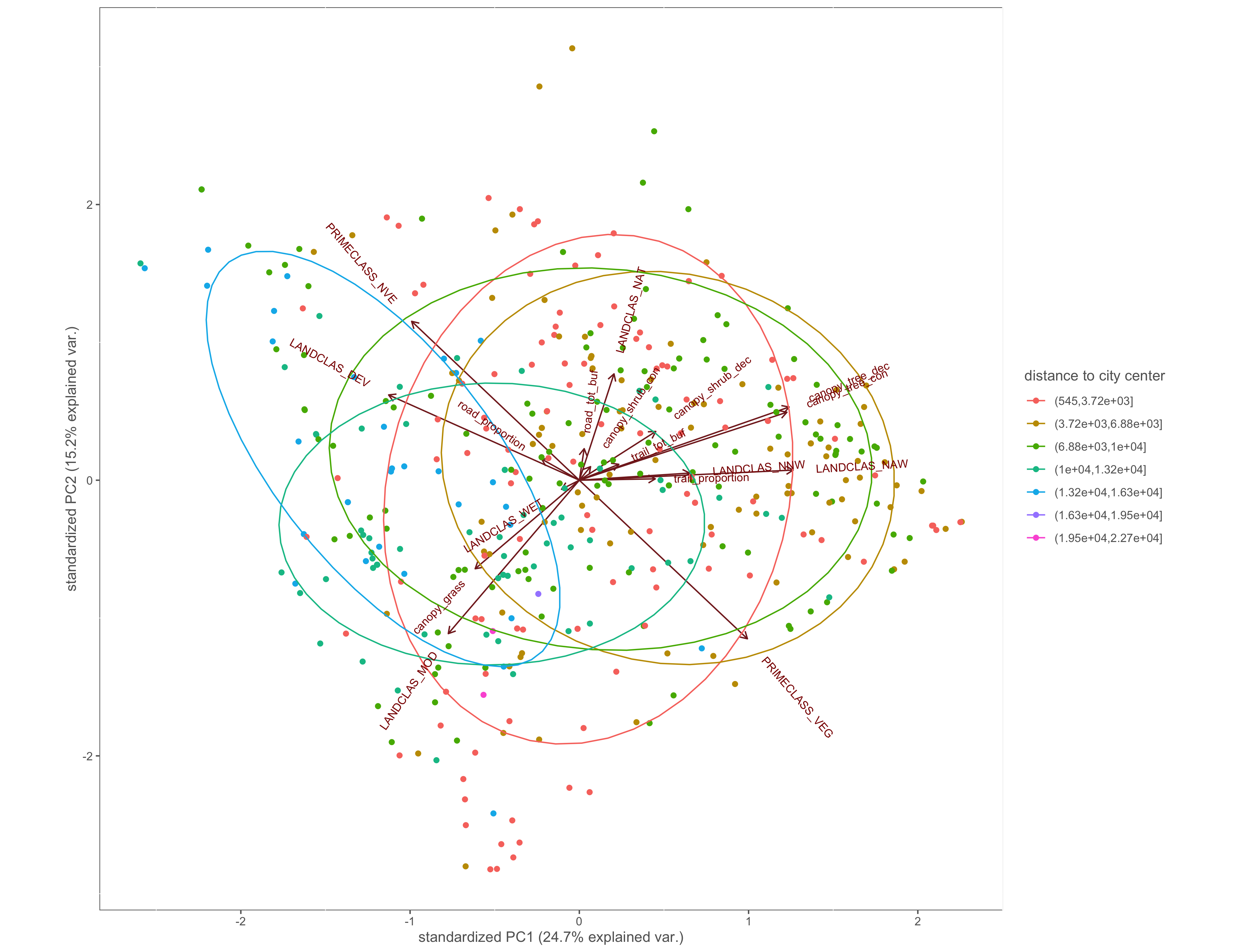
Figure 4.8: PCA biplot with pinch-points grouped by the distance to city center
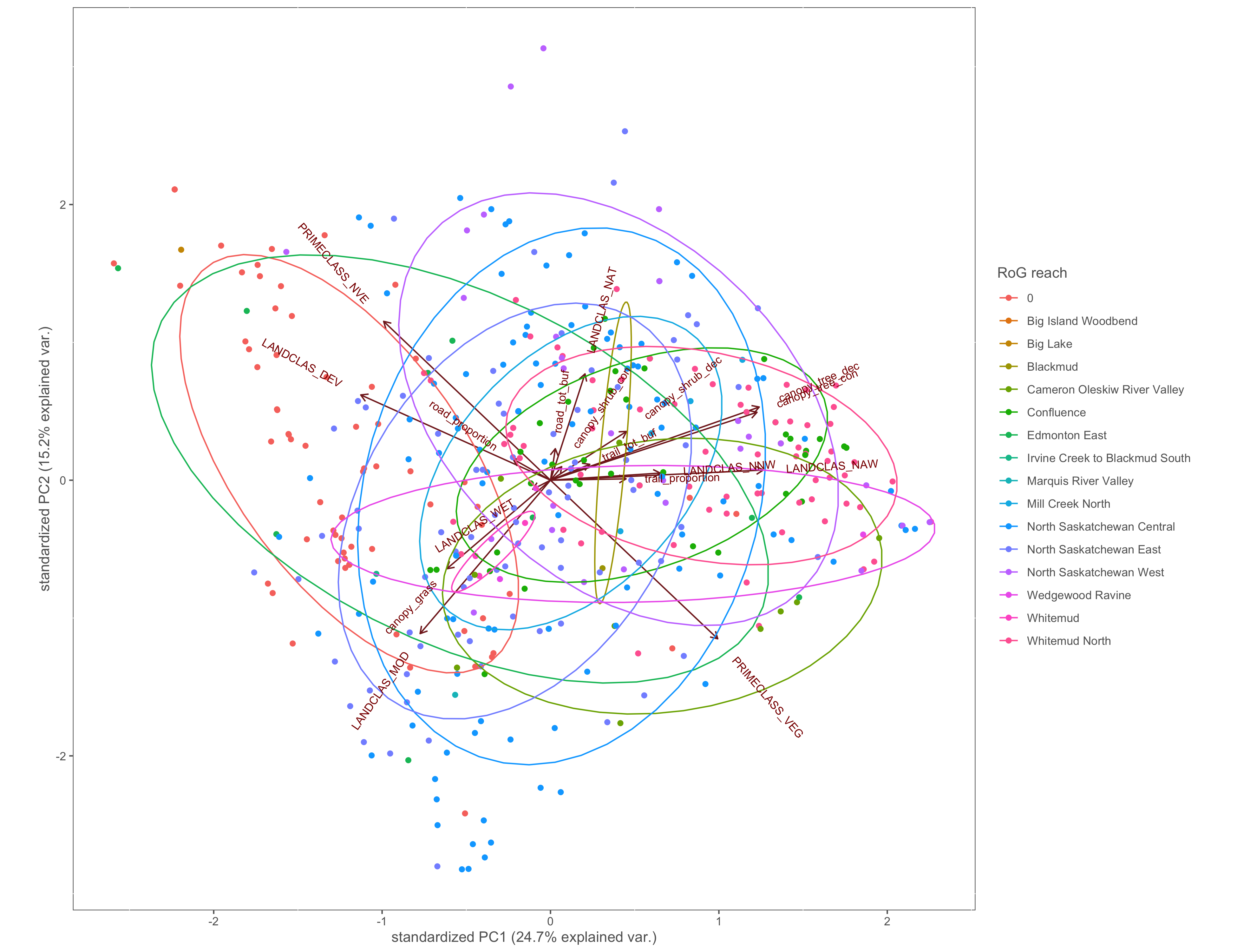
Figure 4.9: PCA biplot with pinch-points grouped by the RoG reach
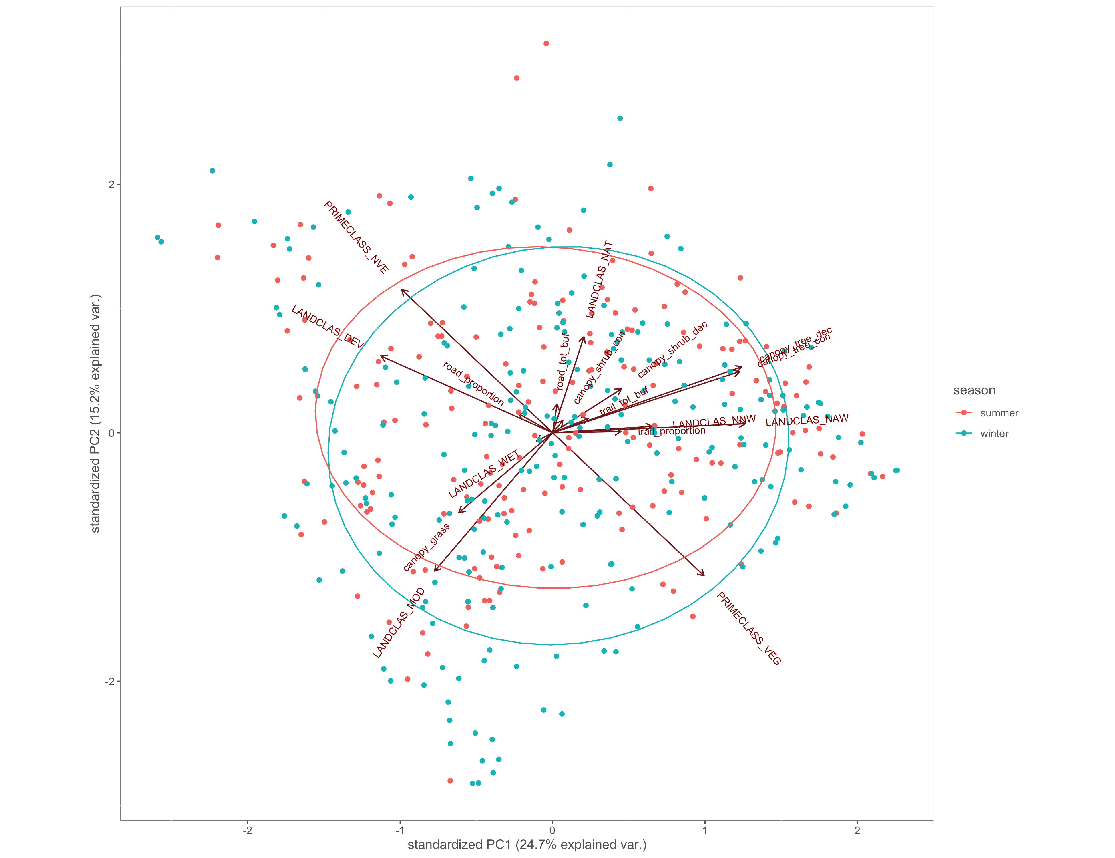
Figure 4.10: PCA biplot with pinch-points grouped by season
hierarchical clustering of PCA
#hc<-hclust(dist(x.pca_2$loadings))

loadings = x.pca$loadings[]

    q = loadings[,1]
    y = loadings[,2]
    z = loadings[,3]


    hc = hclust(dist(cbind(q,y)), method = 'ward')

    png("4_output/PCA/hclust_plot", width=1000, height=600)
    plot(hc, axes=F,xlab='', ylab='',sub ='', main='Clusters')
    rect.hclust(hc, k=4, border='red')
    dev.off()


# view clusters in biplot
x.pca2<-x.pca

# pct=paste0(colnames(x.pca2$x)," (",sprintf("%.1f",x.pca2$sdev/sum(x.pca2$sdev)*100),"%)")
p2=as.data.frame(x.pca2$x)


x.pca2$k=factor(cutree(hclust(dist(x), method='ward'),k=3))
ggbiplot(x.pca2,  ellipse=TRUE, groups=x.pca2$k)+
  labs(color="cluster")+
    custom_theme()
Figure 4.11: Hierarchical clusters of PCA variables
Sort pinch-points into coresponding clusters
# Compute hierarchical clustering on principal components

# Compute PCA with ncp = 3.  The argument ncp = 3 is used in the function PCA() to keep only the first three principal components.
res.pca <- PCA(x[,c(12:28)], ncp = 3, graph = FALSE)
save(res.pca, file="3_pipeline/store/res_pca.rData" )

res.hcpc <- HCPC(res.pca, graph = FALSE)
save(res.hcpc, file="3_pipeline/store/res_hcpc.rData" )


# res.hcpc.var <- HCPC(res.pca$var$coord, graph = TRUE)


fviz_dend(res.hcpc,
          cex = 0.7,                     # Label size
          palette = "jco",               # Color palette see ?ggpubr::ggpar
          rect = TRUE, rect_fill = TRUE, # Add rectangle around groups
          rect_border = "jco",           # Rectangle color
          labels_track_height = 0.3      # Augment the room for labels
          )

fviz_cluster(res.hcpc,
             repel = TRUE,            # Avoid label overlapping
             show.clust.cent = FALSE,
             ellipse= FALSE,# Show cluster centers
             palette = "jco",         # Color palette see ?ggpubr::ggpar
             ggtheme = theme_minimal(),
             main = "Factor map"
             )
fviz_pca_biplot(res.pca)

+
#
#   fviz_cluster(res.hcpc,x.pca,
#              repel = TRUE,            # Avoid label overlapping
#              show.clust.cent = TRUE, # Show cluster centers
#              palette = "jco",         # Color palette see ?ggpubr::ggpar
#              ggtheme = theme_minimal(),
#              main = "Factor map"
#              )
#     ggbiplot(x.pca, circle = TRUE)


#Visualize on biplot
  hcpc_biplot<-ggbiplot(x.pca,  ellipse=TRUE, groups=res.hcpc$data.clust$clust, varname.size = 3)+
  scale_color_manual(name="Cluster", values=c("#1b9e77", "#d95f02", "#7570b3", "#e7298a"))+
  coord_cartesian(clip = "off")+
  custom_theme()

  ggsave(filename="4_output/PCA/pca_cluster_group.png", width = 13, height = 10)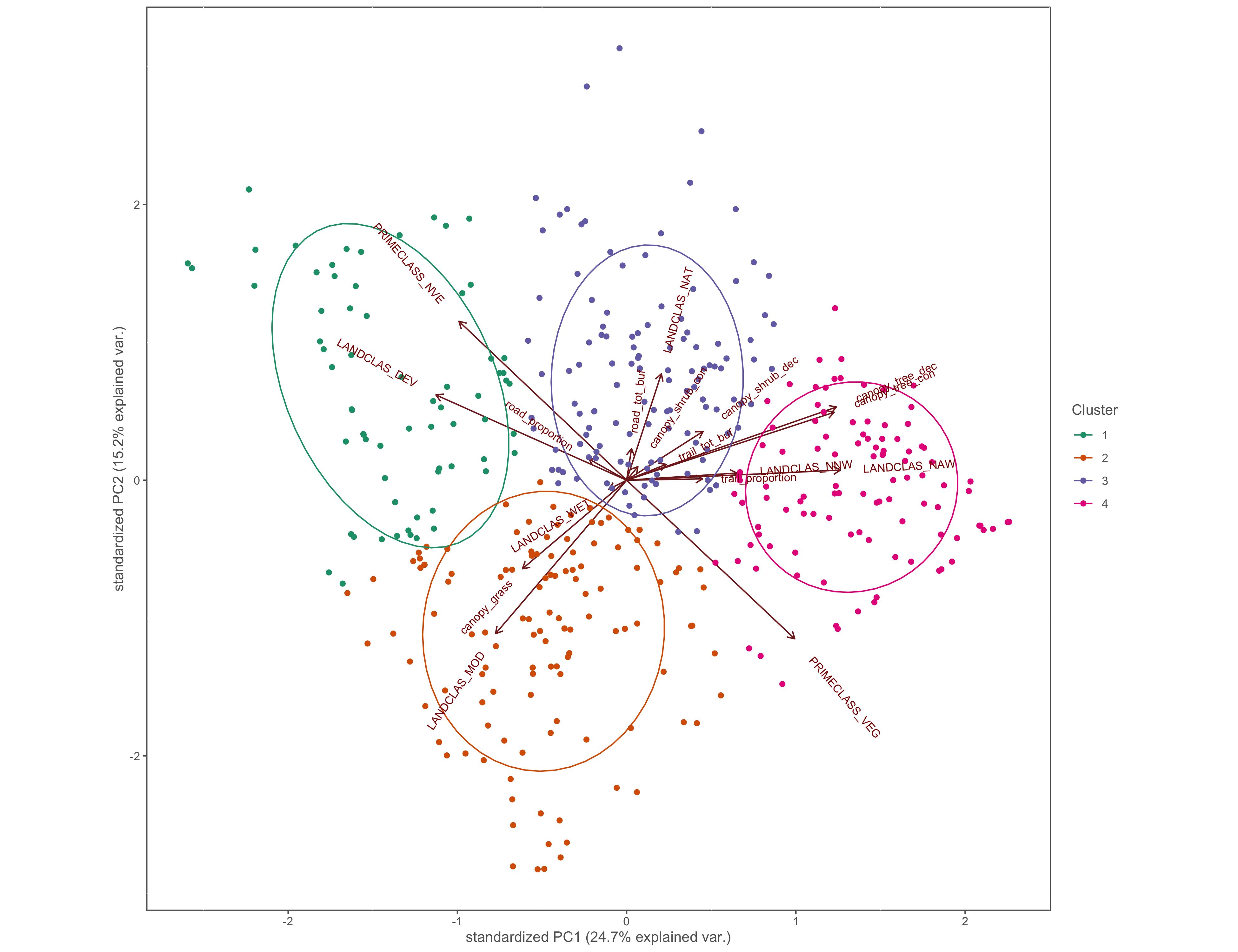
Figure 4.12: PCA biplot with pinch-points grouped by hierarchical cluster
Plot clustered points onto a map
#make a data frame with pinch-point id and cluster

pp_clus<-as.data.frame(res.hcpc$data.clust)
pp_clus <- tibble::rownames_to_column(pp_clus, "group")
pp_clus<- pp_clus[c(1,19)]
save(pp_clus, file="3_pipeline/tmp/pp_clus.rData")


#plot distribution

custom_theme<-function(){theme(
        panel.background = element_rect(fill = "white", color="#636363"),
        # axis.line.y = element_line(colour = "#636363"),
        axis.text.y = element_text(colour="#636363"),
        axis.ticks.y = element_line(colour = "#636363"),
        axis.title.y = element_text(colour="#636363"),
        axis.text.x = element_text(colour="#636363"),
        axis.ticks.x = element_line(colour = "#636363"),
        #axis.line.x = element_line(colour = "#636363"),
        axis.title.x = element_text(colour="#636363"),
        legend.title = element_text(colour="#636363"),
        legend.text = element_text(colour="#636363"),
        legend.key = element_rect(fill = "white"),
      panel.grid.major = element_line(size = 0.0, colour="#bdbdbd"),
      aspect.ratio = 5/5
        #panel.grid.minor = element_line(size = 0.0)
)}

d<-ggplot(data=pp_clus, aes(x=clust))+
  xlab("pinch-point cluster")+
  geom_bar(stat="count")+
custom_theme()
d


# load sf object with pinch-point polygons
load("1_data/manual/pp_all_clus_RoG_wgs.rdata")

pp_all_clus_RoG_wgs_clus<-left_join(pp_all_clus_RoG_wgs, pp_clus)%>%
  rename(hcpc_clust=clust)


save(pp_all_clus_RoG_wgs_clus, file="1_data/manual/pp_all_clus_RoG_wgs_clus.rdata")
Entire city
library(tmap)
library(tmaptools)
library(gridExtra)


# summer only pinch-points
sum_pp<-pp_all_clus_RoG_wgs_clus %>% filter(season=="summer")
# load ribbon of green
RoG_Reaches<-st_read("1_data/external/Ribbon_of_Green_Study_Area_Reaches/Reach_Boundaries/RoG_Reaches_V1_210301/RoG_Reaches_V1_210301.shp")
# check crs
st_crs(RoG_Reaches)
# NAD83_3TM_114_Longitude_Meter_Province_of_Alberta_Canada
RoG_Reaches<-st_transform(RoG_Reaches, crs = st_crs(3776))


# load city boundary
City_Boundary<-st_read("1_data/external/City_Boundary/City_Boundary.shp")

# reproject to match the CRS of RoG_reaches
City_Boundary<-st_transform(City_Boundary, crs = st_crs(3776))

#load road data
v_road<-st_read("1_data/external/roads_data/V_ROAD_SEGMENT_CUR.shp")
# reproject to match the CRS of RoG_reaches
v_road<-st_transform(v_road, crs = st_crs(3776))

# crop roads file by a bounding box of the north saskatchewan central region polygon
v_road_1<-st_crop(v_road, City_Boundary)


bbox_RoG<-st_bbox(RoG_Reaches)%>%
  st_as_sfc()

#plot shape file

pal=c("#1b9e77" , "#d95f02", "#7570b3", "#e7298a")
m<-
  tm_shape(bbox_RoG)+
    tm_borders(col="white")+
  tm_shape(City_Boundary)+tm_borders(col = "#636363")+tm_fill(col="#d9d9d9")+
  tm_layout(frame=FALSE, legend.text.size=.5, legend.width=2, legend.position=c("left","bottom"),)+
  tm_legend(outside=TRUE, frame=FALSE)+
  tm_shape(v_road_1)+tm_lines(col="white", lwd = .8)+
    tm_shape(City_Boundary)+
    tm_borders(col="#636363")+
    tm_fill(col="white", alpha = .5)+
  tm_shape(RoG_Reaches)+
   tm_fill(col="#8bd867", alpha = .3)+
   tm_borders(col = "#636363", lwd = 0)+
  tm_shape(sum_pp)+
   tm_fill(col="hcpc_clust", palette=pal, contrast = c(0.26, 1),alpha = 1, title="Pinch-point clusters", labels = c("1: LANDCLASS DEV, PRIMECLASS_NVE","2: LANDCLASS_MOD, canopy_grass, LANDCLASS_WET","3: LANDCLASS_NAT, canopy_shrub","4: canopy_tree, LANDCLAS_NAW, LANDCLAS_NNW"))+
   tm_borders(col = "#636363", lwd = 0)+
  tm_layout(frame=TRUE, legend.show = TRUE, legend.outside=FALSE, legend.bg.color = "white", legend.text.size = .6, legend.position = c("left", "top"))
m


t_grob<-tmap_grob(m)
g1<-arrangeGrob(t_grob)

lay2 <- cbind(c(1),
              c(1),
              c(1),
              c(2),
              c(2))

g3<-arrangeGrob(g1, hcpc_biplot, layout_matrix =lay2)

ggsave("4_output/maps/pp_hclust_map2.png", g3, width=15, height=9)

tmap_save(m, "4_output/maps/pp_hclust_map.png", outer.margins=c(0,0,0,0))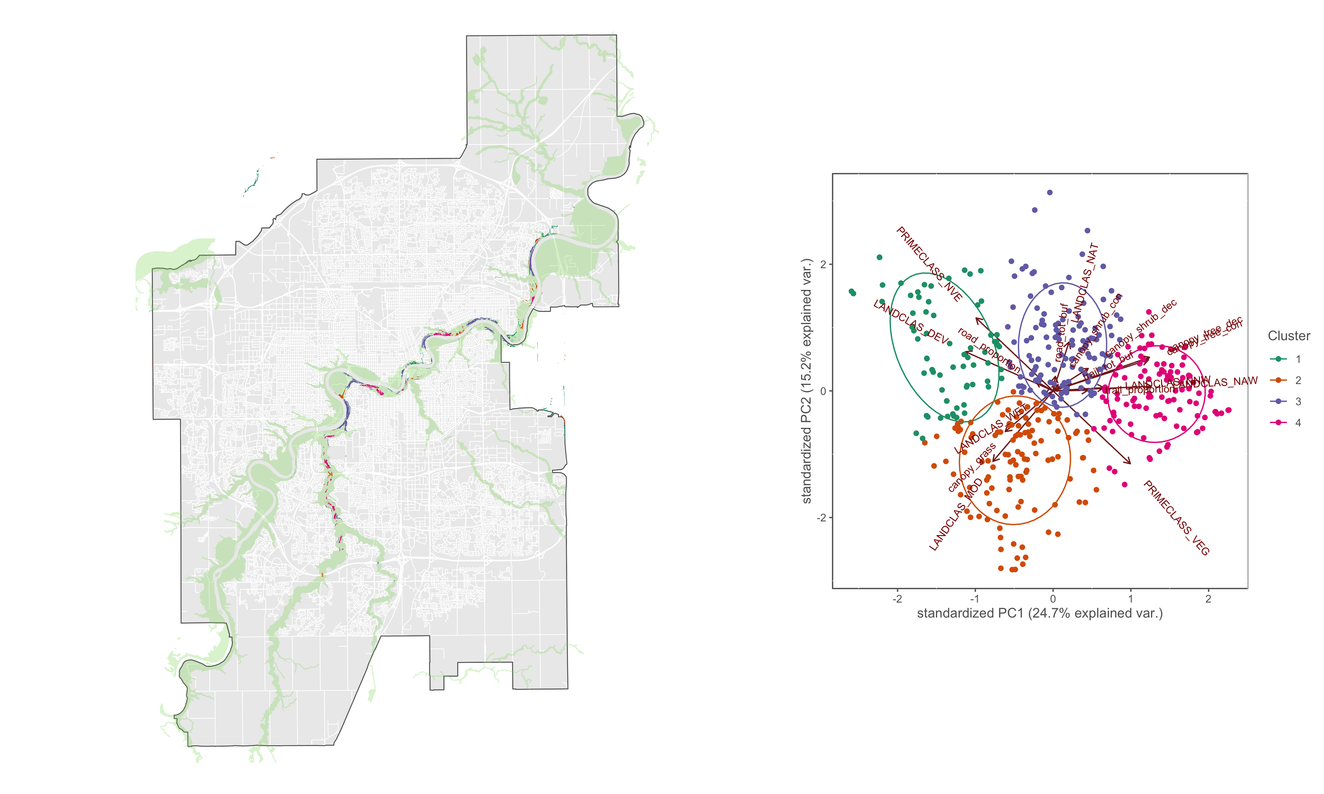
Figure 4.13: Pich-points sorted by hierarchical cluster
Central reach
load("1_data/manual/study_area.rdata")

# load clipped road data
load("1_data/manual/v_road_clip.rdata")

# load polygon representing North Central Region of Saskatchewan region of the ribbon of green
load("1_data/manual/nscr.rdata")


m1<-
  tm_shape(v_road_clip)+tm_lines(col="white")+
  tm_layout(bg.col="#d9d9d9")+
  tm_shape(nscr)+
    tm_fill(col="white", alpha=.4)+
    tm_borders(col = "#636363")+
 tm_shape(sum_pp)+
   tm_fill(col="hcpc_clust", palette=pal, contrast = c(0.26, 1),alpha = 1, title="Hierarchical clusters", labels = c("1: LANDCLASS DEV, PRIMECLASS_NVE","2: LANDCLASS_MOD, canopy_grass, LANDCLASS_WET","3: LANDCLASS_NAT, canopy_shrub","4: canopy_tree, LANDCLAS_NAW, LANDCLAS_NNW"))+
   tm_borders(col = "#636363", lwd = 0)+
  tm_layout( legend.show = TRUE, legend.bg.color = "white", legend.text.size = .6, legend.frame.lwd = 1, legend.frame = "black")
m1

tmap_save(m1, "4_output/maps/pp_hclust_map_NSC.png", outer.margins=c(0,0,0,0))

t_grob<-tmap_grob(m1)
g2<-arrangeGrob(t_grob)

lay2 <- rbind(c(1),
              c(1),
              c(1),
              c(1),
              c(2),
              c(2),
              c(2),
             c(2),)
v
g4<-arrangeGrob(g3, g2, layout_matrix =lay2)

ggsave("4_output/maps/pp_hclust_map2_NSC.png", g4, width=19, height=17)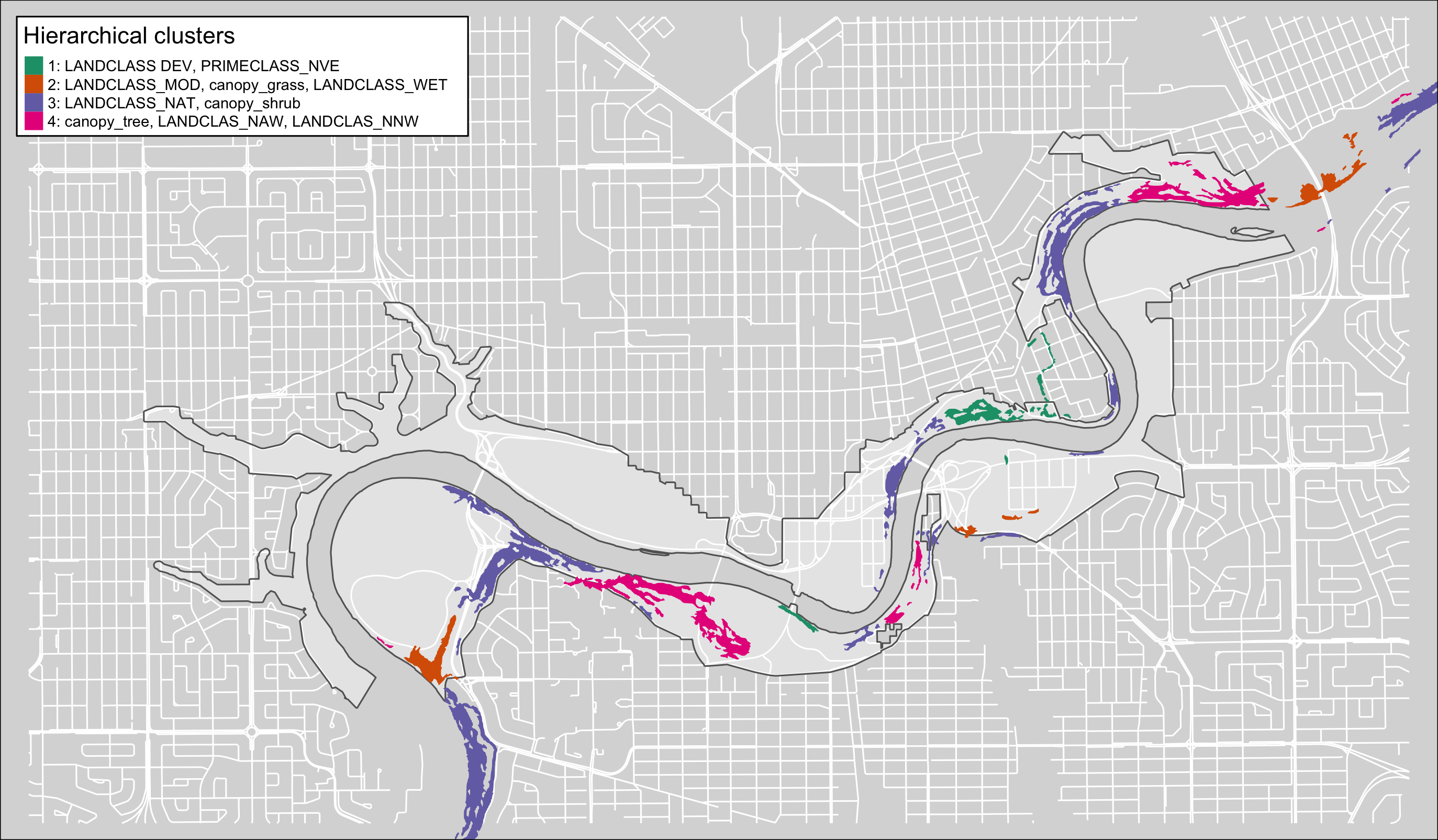
Figure 4.14: Pinch-points sorted by hierarchical cluster in the North Saskatchewan Central reach of the Ribbon of Green.