Proximity
library(sf)
library(dplyr)
library(raster)
library(tmap)
library(ggplot2)
library(gridExtra)
library(scales)
Load data
Biophisical data
Load prepared and clipped biophysical layers.
Pinch-points
Load buffered pinch-point polygons
# buffered pinch point polygons
load("3_pipeline/store/pp_s_clip_clus_buf_ext.rData")

# pinch point clusters
load("3_pipeline/tmp/pp_s_clip_clus.rData")

#calculate area of pinch point polygons
pp_s_clip_clus$pp_area<-st_area(pp_s_clip_clus)

# buffered pinchpoints
load("3_pipeline/store/pp_s_clip_clus_buf.rData")Roads
#transform pinch-point polygon shape to line
pp_s_clip_clus_boundary <- st_cast(pp_s_clip_clus,"MULTILINESTRING")

dist<-st_distance(pp_s_clip_clus_boundary, road_ws_clip)
n<-nearest(dist)

# ddmin <- apply(d, 2, min)
# x<-pp_s_clip_clus
# x$roadDist<-dmin

#create a data.frame with the distance and the coordinates of the points
df <- data.frame(dist=as.vector(dist)/1000,
                    st_coordinates(road_ws_clip))
df<-data.frame(dist)
#structure
str(df)
## 'data.frame':    4104 obs. of  3 variables:
##  $ dist: num  0.791 1.151 1.271 3.129 2.429 ...
##  $ X   : num  608796 613796 583796 588796 593796 ...
##  $ Y   : num  7033371 7033371 7038371 7038371 7038371 ...
#colors


col_dist <- brewer.pal(11,"RdGy")


ggplot(df,aes(X,Y,fill=dist)) #variables
         geom_tile()+ #geometry
           scale_fill_gradientn(colours=rev(col_dist))+ #colors for plotting the distance
             labs(fill="Distance (km)")+ #legend name
             theme_void()+ #map theme
              theme(legend.position = "bottom") #legend position
Total length of roads in pinch-points
########## just in buffer ############
polys_buf<-pp_s_clip_clus_buf_ext

int_buf = st_intersection(road_ws_clip, polys_buf)

plot(polys_buf$geom)
plot(int_buf$geom, lwd = 2, add = TRUE)

#Get the total length of road within each polygon. (polygons with no lines are missing from list)
road_tot_buf<-tapply(st_length(int_buf), int_buf$ID.1,sum)

polys_buf$road_tot_buf = rep(0,nrow(polys_buf))
polys_buf$road_tot_buf[match(names(road_tot_buf),polys_buf$ID)] = road_tot_buf

plot(polys_buf[,"road_tot_buf"])
save(polys_buf, file = "3_pipeline/tmp/polys_buf.rData")


########## just in pinch-point cluster ############
polys_pp<-pp_s_clip_clus

int_pp = st_intersection(road_ws_clip, polys_pp)

plot(polys_pp$geom)
plot(int_pp$geom, lwd = 2, add = TRUE)

#Get the total length of road within each polygon. (polygons with no lines are missing from list)
road_tot_pp<-tapply(st_length(int_pp), int_pp$group,sum)

polys_pp$road_tot_pp = rep(0,nrow(polys_pp))
polys_pp$road_tot_pp[match(names(road_tot_pp),polys_pp$group)] = road_tot_pp

plot(polys_pp[,"road_tot_pp"])
save(polys_pp, file = "3_pipeline/tmp/polys_pp.rData")


########## pp and buffer ############
polys_pp_buf<-pp_s_clip_clus_buf

int_pp_buf = st_intersection(road_ws_clip, polys_pp_buf)

plot(polys_pp_buf$geom)
plot(int_pp_buf$geom, lwd = 2, add = TRUE)

#Get the total length of road within each polygon. (polygons with no lines are missing from list)
road_tot_pp_buf<-tapply(st_length(int_pp_buf), int_pp_buf$group,sum)

polys_pp_buf$road_tot_pp_buf = rep(0,nrow(polys_pp_buf))
polys_pp_buf$road_tot_pp_buf[match(names(road_tot_pp_buf),polys_pp_buf$group)] = road_tot_pp_buf

plot(polys_pp_buf[,"road_tot_pp_buf"])

save(polys_pp_buf, file = "3_pipeline/tmp/polys_pp_buf.rData")

road_tot<-cbind(polys_pp, polys_buf, polys_pp_buf)

road_tot<-road_tot[-c(2,4, 5,7)] #trail_tot<-trail_tot[-c(2,4, 5,7)]


save(road_tot,file="3_pipeline/store/road_tot.rData")| group | pp_area | road_tot_pp | ID |
|---|---|---|---|
| 1 | 56732.587 | 0.00000 | 1 |
| 2 | 147058.199 | 345.33855 | 2 |
| 3 | 143778.108 | 339.33595 | 3 |
| 4 | 9827.057 | 0.00000 | 4 |
| 5 | 10188.943 | 24.01242 | 5 |
| 6 | 34842.657 | 172.97255 | 6 |
| 7 | 9864.212 | 0.00000 | 7 |
| 8 | 107870.712 | 100.65931 | 8 |
| 9 | 6456.471 | 135.02641 | 9 |
| 10 | 12542.062 | 0.00000 | 10 |
| 11 | 89517.780 | 0.00000 | 11 |
| 12 | 10441.776 | 0.00000 | 12 |
| 13 | 46248.183 | 0.00000 | 13 |
| 14 | 8006.357 | 0.00000 | 14 |
Proportion of pinch point within set distance to a road
# Compute a 50 meter buffer around roads in Edmonton
r_buf<-st_buffer(road_ws_clip, dist = 50, singleSide = FALSE)

#intersect
r_buf_int<-st_intersection(r_buf, pp_s_clip_clus)
r_buf_int$r_area<-st_area(r_buf_int)


x<-r_buf_int

#dissolve pilygons by group # and calculate area for each group
x_dis <- x %>% group_by(group) %>% summarize()
#x_dis$r_area<-st_area(nc_dissolve)
x_dis$r_area<-st_area(x_dis)

#add the area for the pinch-points
x_dis<-left_join(x_dis, as.data.frame(pp_s_clip_clus))

#calculate proportion of polygon within distance of a road
x<-x_dis
prop_Road<-as.data.frame(x) %>%
  group_by(group)%>%
  summarize(pp_area=mean(pp_area), r_area=sum(r_area) )%>%
  mutate(proportion=r_area/pp_area)

save(prop_Road, file="3_pipeline/store/prop_Road.rData")| group | pp_area | r_area | proportion |
|---|---|---|---|
| 1 | 56732.587 | 1706.7440 | 3 |
| 2 | 147058.199 | 65773.6153 | 45 |
| 3 | 143778.108 | 34331.4359 | 24 |
| 4 | 9827.057 | 3999.6955 | 41 |
| 5 | 10188.943 | 2581.5991 | 25 |
| 6 | 34842.657 | 20439.8212 | 59 |
| 7 | 9864.212 | 127.4521 | 1 |
| 8 | 107870.712 | 11008.4475 | 10 |
| 9 | 6456.471 | 6456.4708 | 100 |
| 10 | 12542.062 | 8528.9136 | 68 |
| 11 | 89517.780 | 2854.0675 | 3 |
| 12 | 10441.776 | 1131.7581 | 11 |
| 13 | 46248.183 | 329.9234 | 1 |
| 14 | 8006.357 | 4392.5352 | 55 |
Attributes of intersecting roads
int_road_attr<-as.data.frame(int_pp_buf)[c("ID", "group", "LANE_WIDTH", "SPEED")]
save(int_road_attr, file="3_pipeline/tmp/int_road_attr.rData")| ID | group | LANE_WIDTH | SPEED | |
|---|---|---|---|---|
| 21674 | 9862 | 1 | 7.0 | 50 |
| 25632 | 23541 | 1 | 8.9 | 60 |
| 235 | 77175 | 2 | 5.2 | 50 |
| 2837 | 23517 | 2 | 6.1 | 50 |
| 2838 | 77169 | 2 | 6.1 | 50 |
| 2839 | 23077 | 2 | 6.7 | 50 |
| 4022 | 30515 | 2 | 6.0 | 50 |
| 5625 | 12262 | 2 | 8.0 | 50 |
| 6610 | 12305 | 2 | 8.0 | 50 |
| 6611 | 77180 | 2 | 5.0 | 50 |
| 6613 | 2190 | 2 | 8.0 | 50 |
| 6614 | 24603 | 2 | 8.0 | 50 |
| 6618 | 51421 | 2 | 9.1 | 50 |
| 9130 | 38119 | 2 | 5.5 | 50 |
| 10054 | 23075 | 2 | 6.8 | 50 |
| 15163 | 12309 | 2 | 9.0 | 50 |
| 15299 | 23457 | 2 | 7.1 | 50 |
| 16634 | 62567 | 2 | 4.5 | 50 |
| 24424 | 30495 | 2 | 6.1 | 50 |
| 25617 | 19837 | 2 | 7.3 | 60 |
| 25633 | 23559 | 2 | 6.8 | 60 |
| 25634 | 3917 | 2 | 8.7 | 60 |
| 26441 | 23395 | 2 | 8.3 | 60 |
| 26443 | 19836 | 2 | 7.3 | 60 |
| 26451 | 18879 | 2 | 9.0 | 60 |
| 26452 | 18880 | 2 | 7.3 | 60 |
| 27008 | 62565 | 2 | 6.0 | 50 |
| 27779 | 23079 | 2 | 9.3 | 50 |
| 27780 | 23439 | 2 | 6.0 | 50 |
| 6618.1 | 51421 | 3 | 9.1 | 50 |
| 17065 | 26945 | 3 | 10.4 | 50 |
| 17076 | 2825 | 3 | 7.3 | 50 |
| 26841 | 18835 | 3 | 7.6 | 50 |
| 7579 | 12652 | 4 | 9.0 | 50 |
| 22855 | 12651 | 4 | 9.1 | 50 |
| 15778 | 3652 | 5 | 7.3 | 50 |
| 26843 | 2626 | 5 | 9.0 | 50 |
| 1015 | 23379 | 6 | 4.9 | 50 |
| 7287 | 17558 | 6 | 8.4 | 50 |
| 7289 | 23383 | 6 | 8.6 | 50 |
| 7290 | 3547 | 6 | 11.3 | 50 |
| 8888 | 23767 | 6 | 12.4 | 60 |
| 9145 | 23765 | 6 | 12.1 | 60 |
| 9146 | 23755 | 6 | 14.0 | 60 |
| 10400 | 17547 | 6 | 7.3 | 50 |
| 11859 | 19845 | 6 | 6.7 | 50 |
| 12295 | 23757 | 6 | 12.4 | 60 |
| 13941 | 19844 | 6 | 6.9 | 50 |
| 16174 | 8247 | 6 | 13.0 | 30 |
| 16175 | 8248 | 6 | 7.9 | 50 |
| 16185 | 4606 | 6 | 7.9 | 50 |
| 21846 | 442 | 6 | 11.0 | 50 |
| 26670 | 1813 | 6 | 9.1 | 30 |
| 27864 | 23375 | 6 | 5.9 | 50 |
| 30255 | 24483 | 6 | 7.3 | 50 |
| 29853 | 20062 | 8 | 6.2 | 50 |
| 6046 | 19290 | 9 | 9.0 | 50 |
| 11858 | 19284 | 9 | 7.3 | 60 |
| 11860 | 19283 | 9 | 7.7 | 60 |
| 13938 | 19281 | 9 | 12.0 | 60 |
| 13940 | 19282 | 9 | 10.3 | 60 |
| 27058 | 19288 | 9 | 6.4 | 50 |
| 10751 | 4665 | 10 | 9.0 | 50 |
| 29824 | 5551 | 10 | 8.2 | 50 |
| 29851 | 5652 | 10 | 7.3 | 50 |
| 4936 | 5820 | 11 | 7.9 | 50 |
| 626 | 20072 | 12 | 7.0 | 50 |
| 7291 | 2709 | 14 | 8.6 | 50 |
Create distance to road raster
load("1_data/manual/study_area.rData")

# shp<-study_area
#
# grid <- shp %>%
#   st_make_grid(cellsize = 10, what = "centers") #%>% # grid of points
#   #st_intersection(shp)                               #
#
# d = st_distance(grid, road_ws_clip, byid=TRUE)

######

lines<-road_ws_clip$geometry
#lines<-st_union(lines)

plot(lines)

r = raster(extent(study_area),400,400)
crs(r)<-crs(lines)

#r<-crs(r, crs="+init=ESPG:3776")
#(rgeos)
p = as(r,"SpatialPoints")
p<-st_as_sf(p)

#d=gDistance(p, lines)
d=st_distance(p, lines)
dim(d)
dmin=apply(d, 1, min)
r[]=dmin


save(r, file="3_pipeline/tmp/dist2road.rData")
Summarize distance to road pixels
load("3_pipeline/tmp/dist2road.rData")

poly<-pp_s_clip_clus_buf_ext
#poly$ID <- 1:length(poly)
poly$layer <- NULL
d <- data.frame(poly)
v<-extract(r,  poly, na.rm=TRUE, df=TRUE)

vd <- merge(d, v, by="ID")
vd %>%
  rename(minDist=layer)

names(vd)[names(vd) == "layer"] <- "minDist"

#vd<- vd[-c(3)]
#save(vd, file="3_pipeline/tmp/vd.rData")


##### plot ###########

m4<-
  tm_shape(r$layer)+
    tm_raster(palette = c("#7fcdbb", "#253494"),
      title = "Distance to road (m)",
              contrast = c(0,.8),
              style = "cont")+
   tm_shape(road_ws_clip)+tm_lines(col="#ffffd9")+
  #tm_layout(bg.col="#d9d9d9")+
  tm_shape(nscr)+
    #tm_fill(col="white", alpha=.4)+
    tm_borders(col = "#636363")+
  tm_shape(pp_s_clip_clus)  +
    #tm_fill(col="MAP_COLORS", palette = "Dark2", alpha=.8)+
    tm_borders(alpha=1)+
   tm_shape(pp_s_clip_clus_buf)+
    tm_text(text = "group",
          col="black",
          size = 1.3)+
  tm_layout(legend.outside = FALSE,
            legend.text.size = .8,
            legend.bg.color="white",
            legend.frame=TRUE,
            legend.title.size=1,
            legend.frame.lwd=.8,
            )
m4

#convert tmap to grob
g1<-tmap_grob(m4)

# create hist plots in ggplot convert to grob objects which will be plotted in tmap.
g2<-vd%>%
    ggplot(aes(x = minDist)) +
    geom_histogram(binwidth=1, position = "identity", aes(y=..ncount..), fill="#00441b") +
  #geom_density(alpha=.2, fill="#FF6666")+
    scale_y_continuous(labels = percent_format())+
    #scale_x_continuous()+
  labs(x="distance 2 road", y="% count")+
    theme(#panel.background = element_blank(),
          axis.ticks=element_blank(),
          strip.background =element_rect(fill="white"),
          panel.background = element_rect(fill="#ece2f0"),
          panel.grid.major = element_blank(),
          panel.grid.minor = element_blank())+
    facet_grid(~ID)
  # geom_vline(aes(xintercept=grp.mean),
  #           color="blue", linetype="dashed", size=1)+
g2


lay2 <- rbind(c(1),
              c(1),
              c(1),
              c(1),
              c(2))

m2<-arrangeGrob(g1, g2, layout_matrix =lay2)

ggsave("4_output/maps/summary/distRoad_hist_map.png", m2, width=15, height=12)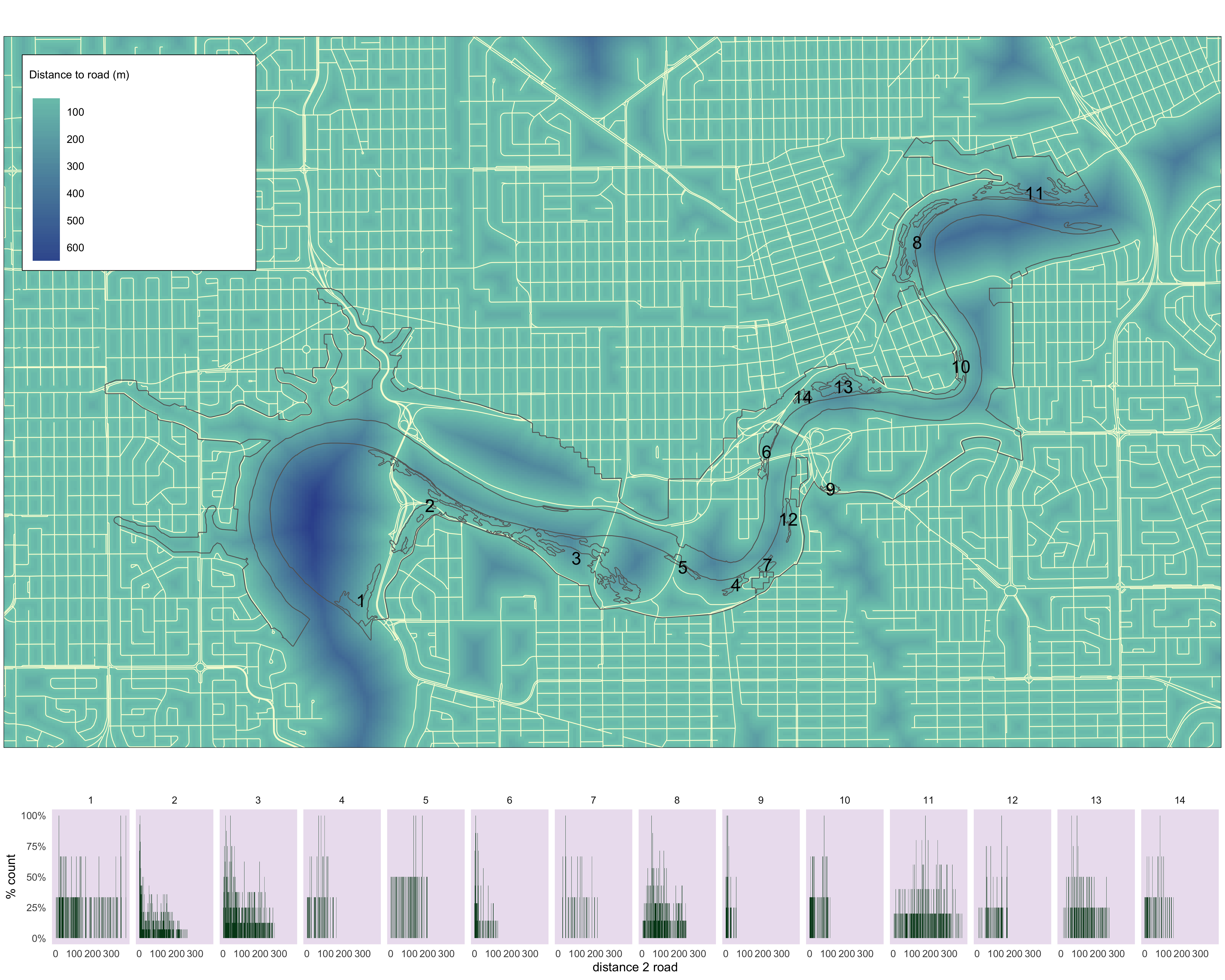
Figure 3.6: Histograms of distance to road values for each pinch point.
Trails
Total length of trails in pinch-points
########## just in buffer ############
polys_buf<-pp_s_clip_clus_buf_ext

int_buf = st_intersection(trails_clip, polys_buf)

plot(polys_buf$geom)
plot(int_buf$geom, lwd = 2, add = TRUE)

#Get the total length of trail within each polygon. (polygons with no lines are missing from list)
trail_tot_buf<-tapply(st_length(int_buf), int_buf$ID.1,sum)

polys_buf$trail_tot_buf = rep(0,nrow(polys_buf))
polys_buf$trail_tot_buf[match(names(trail_tot_buf),polys_buf$ID)] = trail_tot_buf

plot(polys_buf[,"trail_tot_buf"])
save(polys_buf, file = "3_pipeline/tmp/polys_buf.rData")


########## just in pinch-point cluster ############
polys_pp<-pp_s_clip_clus

int_pp = st_intersection(trails_clip, polys_pp)

plot(polys_pp$geom)
plot(int_pp$geom, lwd = 2, add = TRUE)

#Get the total length of trail within each polygon. (polygons with no lines are missing from list)
trail_tot_pp<-tapply(st_length(int_pp), int_pp$group,sum)

polys_pp$trail_tot_pp = rep(0,nrow(polys_pp))
polys_pp$trail_tot_pp[match(names(trail_tot_pp),polys_pp$group)] = trail_tot_pp

plot(polys_pp[,"trail_tot_pp"])
save(polys_pp, file = "3_pipeline/tmp/polys_pp.rData")


########## pp and buffer ############
polys_pp_buf<-pp_s_clip_clus_buf

int_pp_buf = st_intersection(trails_clip, polys_pp_buf)

plot(polys_pp_buf$geom)
plot(int_pp_buf$geom, lwd = 2, add = TRUE)

#Get the total length of trail within each polygon. (polygons with no lines are missing from list)
trail_tot_pp_buf<-tapply(st_length(int_pp_buf), int_pp_buf$group,sum)

polys_pp_buf$trail_tot_pp_buf = rep(0,nrow(polys_pp_buf))
polys_pp_buf$trail_tot_pp_buf[match(names(trail_tot_pp_buf),polys_pp_buf$group)] = trail_tot_pp_buf

plot(polys_pp_buf[,"trail_tot_pp_buf"])

save(polys_pp_buf, file = "3_pipeline/tmp/polys_pp_buf.rData")

trail_tot<-cbind(polys_pp, polys_buf, polys_pp_buf)

trail_tot<-trail_tot[-c(2,4, 5,7)]

save(trail_tot,file="3_pipeline/store/trail_tot.rData")| group | trail_tot_pp | trail_tot_buf | trail_tot_pp_buf |
|---|---|---|---|
| 1 | 1402.8913 | 907.6308 | 2284.9773 |
| 2 | 1746.2777 | 759.6576 | 2213.7281 |
| 3 | 2071.2571 | 2080.6180 | 3947.2904 |
| 4 | 229.3805 | 274.9608 | 482.4089 |
| 5 | 320.1259 | 345.3875 | 665.5135 |
| 6 | 974.8245 | 413.7000 | 1328.5006 |
| 7 | 263.3064 | 304.0481 | 562.3100 |
| 8 | 3035.3910 | 966.6510 | 3664.6942 |
| 9 | 0.0000 | 241.6127 | 241.6127 |
| 10 | 404.2439 | 145.3653 | 511.6370 |
| 11 | 2455.0704 | 885.4490 | 3180.7222 |
| 12 | 255.5054 | 229.7552 | 490.1105 |
| 13 | 1425.4471 | 1502.9733 | 2656.5463 |
| 14 | 170.9482 | 474.4760 | 572.3995 |
Proportion of pinch point within set distance to a trail
# Compute a 50 meter buffer around roads in Edmonton
t_buf<-st_buffer(trails_clip, dist = 50, singleSide = FALSE)

#intersect
t_buf_int<-st_intersection(t_buf, pp_s_clip_clus)
t_buf_int$t_area<-st_area(t_buf_int)


x<-t_buf_int

#dissolve pilygons by group # and calculate area for each group
x_dis <- x %>% group_by(group) %>% summarize()
x_dis$t_area<-st_area(x_dis)

#add the area for the pinch-points
x_dis<-left_join(x_dis, as.data.frame(pp_s_clip_clus))

#calculate proportion of polygon within distance of a trail
x<-x_dis
prop_trail<-as.data.frame(x) %>%
  group_by(group)%>%
  summarize(pp_area=mean(pp_area), t_area=sum(t_area) )%>%
  mutate(proportion=t_area/pp_area)

save(prop_trail, file="3_pipeline/store/prop_trail.rData")| group | pp_area | t_area | proportion |
|---|---|---|---|
| 1 | 56732.587 | 50089.904 | 88 |
| 2 | 147058.199 | 76347.847 | 52 |
| 3 | 143778.108 | 124467.026 | 87 |
| 4 | 9827.057 | 9822.321 | 100 |
| 5 | 10188.943 | 10158.874 | 100 |
| 6 | 34842.657 | 31924.906 | 92 |
| 7 | 9864.212 | 9520.358 | 97 |
| 8 | 107870.712 | 104735.522 | 97 |
| 9 | 6456.471 | 5175.914 | 80 |
| 10 | 12542.062 | 12011.878 | 96 |
| 11 | 89517.780 | 81318.777 | 91 |
| 12 | 10441.776 | 10267.423 | 98 |
| 13 | 46248.183 | 43473.159 | 94 |
| 14 | 8006.357 | 8006.357 | 100 |
Create distance to trail raster
load("1_data/manual/study_area.rData")

# shp<-study_area
#
# grid <- shp %>%
#   st_make_grid(cellsize = 10, what = "centers") #%>% # grid of points
#   #st_intersection(shp)                               #
#
# d = st_distance(grid, road_ws_clip, byid=TRUE)

######

lines<-trails_clip$geometry
#lines<-st_union(lines)

plot(lines)

r = raster(extent(study_area),400,400)
crs(r)<-crs(lines)

#r<-crs(r, crs="+init=ESPG:3776")
#(rgeos)
p = as(r,"SpatialPoints")
p<-st_as_sf(p)

#d=gDistance(p, lines)
d=st_distance(p, lines)
dim(d)
dmin=apply(d, 1, min)
r[]=dmin


save(r, file="3_pipeline/tmp/dist2trail.rData")
Summarize distance to road pixels
load("3_pipeline/tmp/dist2trail.rData")

poly<-pp_s_clip_clus_buf_ext
#poly$ID <- 1:length(poly)
poly$layer <- NULL
d <- data.frame(poly)
v<-extract(r,  poly, na.rm=TRUE, df=TRUE)

vd <- merge(d, v, by="ID")
vd %>%
  rename(minDist=layer)

names(vd)[names(vd) == "layer"] <- "minDist"

#vd<- vd[-c(3)]
#save(vd, file="3_pipeline/tmp/vd.rData")


##### plot ###########

m4<-
  tm_shape(r$layer)+
    tm_raster(palette = c("#ffffd9","#a5dccf", "#7fcdbb", "#384ccd", "#384ccd", "#253494"),
      title = "Distance to trail (m)",
              contrast = c(0,.8),
              style = "cont")+
   tm_shape(trails_clip)+tm_lines(col="white")+
  #tm_layout(bg.col="#d9d9d9")+
  tm_shape(nscr)+
    #tm_fill(col="white", alpha=.4)+
    tm_borders(col = "#636363")+
  tm_shape(pp_s_clip_clus)  +
    #tm_fill(col="MAP_COLORS", palette = "Dark2", alpha=.8)+
    tm_borders(alpha=1)+
   tm_shape(pp_s_clip_clus_buf)+
    tm_text(text = "group",
          col="black",
          size = 1.3)+
  tm_layout(legend.outside = FALSE,
            legend.text.size = .8,
            legend.bg.color="white",
            legend.frame=TRUE,
            legend.title.size=1,
            legend.frame.lwd=.8,
            )
m4

#convert tmap to grob
g1<-tmap_grob(m4)

# create hist plots in ggplot convert to grob objects which will be plotted in tmap.
g2<-vd%>%
    ggplot(aes(x = minDist)) +
    geom_histogram(binwidth=1, position = "identity", aes(y=..ncount..), fill="#00441b") +
  #geom_density(alpha=.2, fill="#FF6666")+
    scale_y_continuous(labels = percent_format())+
    #scale_x_continuous()+
  labs(x="distance 2 road", y="% count")+
    theme(#panel.background = element_blank(),
          axis.ticks=element_blank(),
          strip.background =element_rect(fill="white"),
          panel.background = element_rect(fill="#ece2f0"),
          panel.grid.major = element_blank(),
          panel.grid.minor = element_blank())+
    facet_grid(~ID)
  # geom_vline(aes(xintercept=grp.mean),
  #           color="blue", linetype="dashed", size=1)+
g2


lay2 <- rbind(c(1),
              c(1),
              c(1),
              c(1),
              c(2))

m2<-arrangeGrob(g1, g2, layout_matrix =lay2)

ggsave("4_output/maps/summary/distTrail_hist_map.png", m2, width=15, height=12)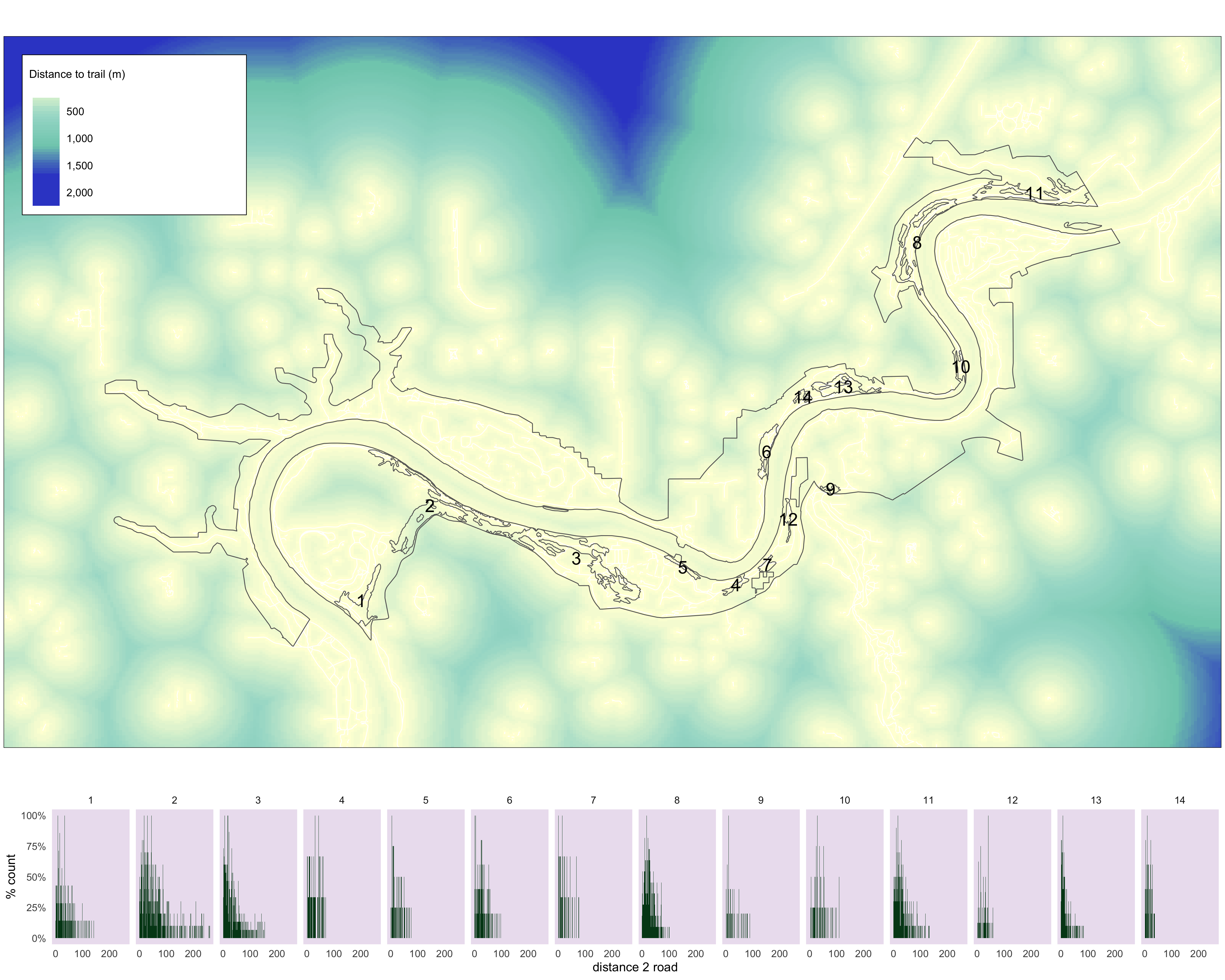
Figure 3.7: Histograms of distance to trail values for each pinch point.