PCA (pinch-point interiors)
Setup
intall libraries
Run PCA
Prep data and run PCA
x<-pp_all_Met_wide_in
x<-x[-c(1,3)]
x<-distinct(x)

rownames(x)<-x[,1]
x<-x[-c(1)]

x$pp_area<-as.numeric(x$pp_area)
x$pp_area<-as.numeric(x$dist2cent)

x[is.na(x)]<-0

#create grouping variable
x$area_group <- cut(x$pp_area, 4)

# x.pca<-prcomp(x[,c(8, 11:27)], center = TRUE, scale. = TRUE)
# summary(x.pca)

x.pca<-princomp(x[,c(11:22)], cor=TRUE)
summary(x.pca)
#print(x.pca$loadings)
save(x.pca, file="3_pipeline/tmp/x.pca_in.rData")

x.pca$scores

#save output as a txt file
sink("4_output/PCA/interior_only/summary_pca.txt")
print(summary(x.pca))
sink()
##
## Loadings:
## Comp.1 Comp.2 Comp.3 Comp.4 Comp.5 Comp.6 Comp.7 Comp.8 Comp.9
## trail_proportion 0.175 0.387 0.213 0.392 0.346 0.128 0.687
## trail_tot 0.274 0.590 -0.614 -0.139 -0.158 -0.375
## road_proportion 0.195 0.521 -0.121 -0.374 0.201 0.262 -0.117 -0.635
## road_tot 0.197 0.576 -0.308 -0.116 0.109 -0.282 0.650
## PRIMECLASS_NVE -0.511 -0.211 0.107
## PRIMECLASS_VEG 0.512 0.208 -0.108
## LANDCLAS_DEV -0.457 0.271 -0.184 -0.311 0.247
## LANDCLAS_MOD -0.128 0.637 -0.240 -0.192 0.269 0.191 -0.107
## LANDCLAS_NAT -0.153 -0.501 -0.236 0.373 0.467 -0.293
## LANDCLAS_NAW 0.395 -0.273 0.132 0.414 -0.171 0.196 -0.201
## LANDCLAS_NNW 0.125 -0.276 0.120 -0.587 -0.239 -0.204 -0.391 0.432
## LANDCLAS_WET -0.112 -0.262 -0.368 0.142 -0.233 0.823 0.161
## Comp.10 Comp.11 Comp.12
## trail_proportion
## trail_tot
## road_proportion
## road_tot
## PRIMECLASS_NVE 0.468 -0.669
## PRIMECLASS_VEG 0.700 0.425
## LANDCLAS_DEV 0.358 0.615
## LANDCLAS_MOD 0.205 -0.555
## LANDCLAS_NAT 0.232 0.402
## LANDCLAS_NAW 0.234 -0.635
## LANDCLAS_NNW 0.112 -0.304
## LANDCLAS_WET
##
## Comp.1 Comp.2 Comp.3 Comp.4 Comp.5 Comp.6 Comp.7 Comp.8 Comp.9
## SS loadings 1.000 1.000 1.000 1.000 1.000 1.000 1.000 1.000 1.000
## Proportion Var 0.083 0.083 0.083 0.083 0.083 0.083 0.083 0.083 0.083
## Cumulative Var 0.083 0.167 0.250 0.333 0.417 0.500 0.583 0.667 0.750
## Comp.10 Comp.11 Comp.12
## SS loadings 1.000 1.000 1.000
## Proportion Var 0.083 0.083 0.083
## Cumulative Var 0.833 0.917 1.000## Importance of components:
## Comp.1 Comp.2 Comp.3 Comp.4 Comp.5
## Standard deviation 1.8546254 1.3038051 1.1719966 1.1077726 1.04100885
## Proportion of Variance 0.2866363 0.1416590 0.1144647 0.1022633 0.09030829
## Cumulative Proportion 0.2866363 0.4282953 0.5427599 0.6450233 0.73533157
## Comp.6 Comp.7 Comp.8 Comp.9 Comp.10
## Standard deviation 0.97562805 0.96131082 0.82741831 0.78419551 2.165611e-02
## Proportion of Variance 0.07932084 0.07700987 0.05705175 0.05124688 3.908227e-05
## Cumulative Proportion 0.81465241 0.89166228 0.94871403 0.99996092 1.000000e+00
## Comp.11 Comp.12
## Standard deviation 2.469117e-08 0
## Proportion of Variance 5.080451e-17 0
## Cumulative Proportion 1.000000e+00 1Visualize eigenvalues (scree plot).
How much variance is explained by each principal componant?
png("4_output/PCA/interior_only/scree_plot", width=1000, height=600)
fviz_eig(x.pca)
dev.off()

# Contributions of variables to PC1
png("4_output/PCA/interior_only/cont_PCA1_plot", width=1000, height=600)
fviz_contrib(x.pca, choice = "var", axes = 1, top = 10)
dev.off()


# Contributions of variables to PC2
png("4_output/PCA/interior_only/cont_PCA2_plot", width=1000, height=600)
fviz_contrib(x.pca, choice = "var", axes = 2, top = 10)
dev.off()
Figure 4.15: Scree plot showing how much variance is explained by each PCA
Figure 4.16: Contribution of variables to Dim-1
Figure 4.17: Contribution of variables to Dim-2
Plot results
# create ggplot theme
custom_theme<-function(){theme(
        panel.background = element_rect( fill = "white", color="#636363"),
        # axis.line.y = element_line(colour = "#636363"),
        axis.text.y = element_text(colour="#636363"),
        axis.ticks.y = element_line(colour = "#636363"),
        axis.title.y = element_text(colour="#636363"),
        axis.text.x = element_text(colour="#636363"),
        axis.ticks.x = element_line(colour = "#636363"),
        #axis.line.x = element_line(colour = "#636363"),
        axis.title.x = element_text(colour="#636363"),
        legend.title = element_text(colour="#636363"),
        legend.text = element_text(colour="#636363"),
        legend.key = element_rect(fill = "white"),
      panel.grid.major = element_line(size = 0.0, colour="#bdbdbd"),
      aspect.ratio = 5/5
        #panel.grid.minor = element_line(size = 0.0)
        )}


# with labels
ggbiplot(x.pca, circle = TRUE)+
  coord_cartesian(clip = "off")+
  custom_theme()
ggsave(filename="4_output/PCA/interior_only/pca.png",  width = 13, height = 10)


#current difference
ggbiplot(x.pca,  ellipse=TRUE, groups=x$cur_diff_group)+
  labs(color="current difference")+
  coord_cartesian(clip = "off")+
    custom_theme()
ggsave(filename="4_output/PCA/interior_only/pca_cur_diff_group.png",  width = 13, height = 10)


#mean current
ggbiplot(x.pca,  ellipse=TRUE, groups=x$cur_in_mean_group)+
  labs(color="Mean current in pinch-point")+
  coord_cartesian(clip = "off")+
    custom_theme()
ggsave(filename="4_output/PCA/interior_only/pca_cur_in_mean_group.png", width = 13, height = 10)


#distance 2 city center
ggbiplot(x.pca,  ellipse=TRUE, groups=x$dist2cent_group)+
  labs(color="distance to city center")+
  coord_cartesian(clip = "off")+
    custom_theme()
ggsave(filename="4_output/PCA/interior_only/pca_dist2cent_group.png", width = 13, height = 10)


#reach
ggbiplot(x.pca,  ellipse=TRUE, groups=x$Reach)+
  labs(color="RoG reach")+
  coord_cartesian(clip = "off")+
    custom_theme()
ggsave(filename="4_output/PCA/interior_only/pca_Reach_group.png", width = 13, height = 10)


#polygon area
ggbiplot(x.pca,  ellipse=TRUE, groups=x$area_group)+
  labs(color="pinch-point area (m)")+
  coord_cartesian(clip = "off")+
    custom_theme()
ggsave(filename="4_output/PCA/interior_only/pca_area_group.png", width = 13, height = 10)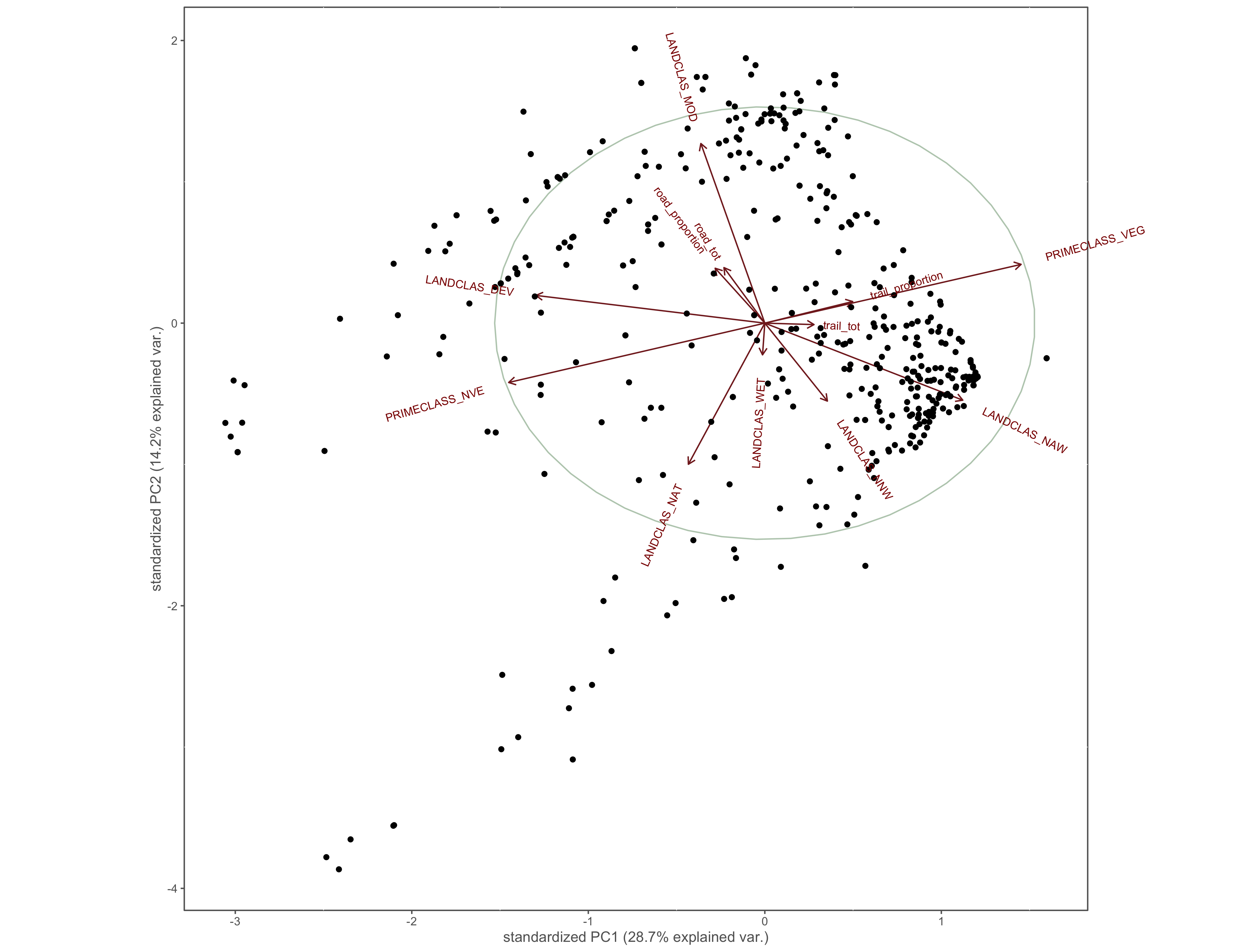
Figure 4.18: PCA results
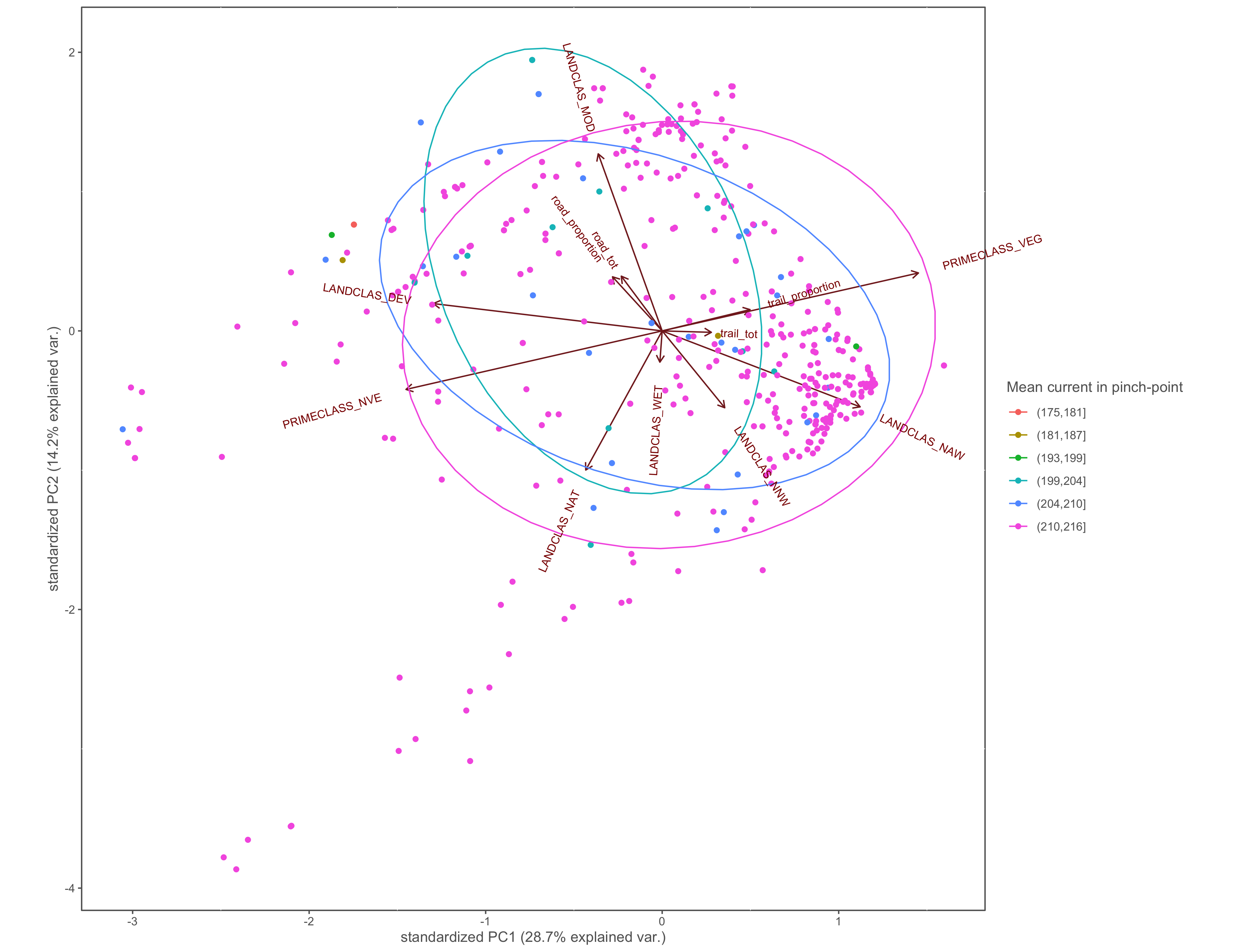
Figure 4.19: PCA biplot with pinch-points grouped by the within pinch-pont mean current values
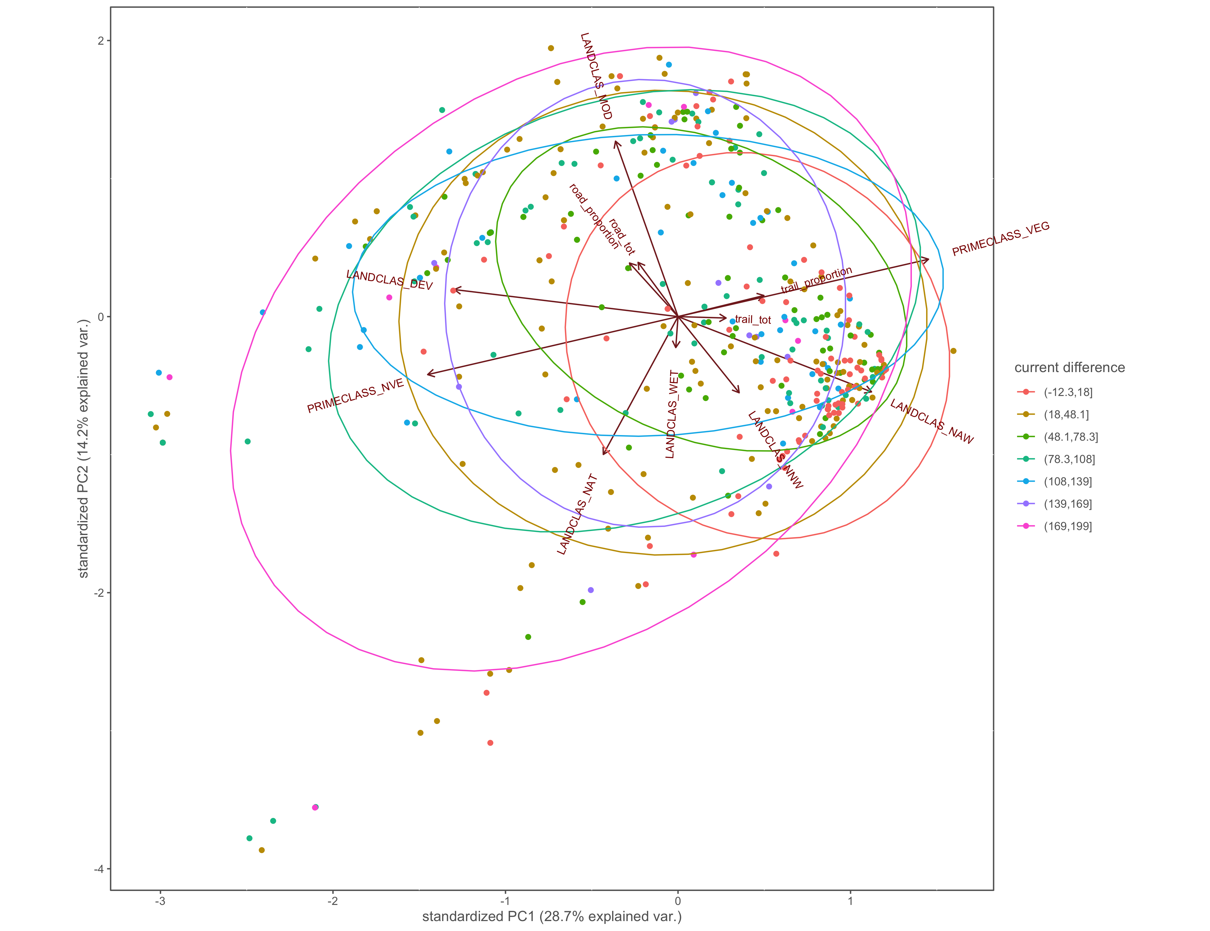
Figure 4.20: PCA biplot with pinch-points grouped by the difference between within and without current values
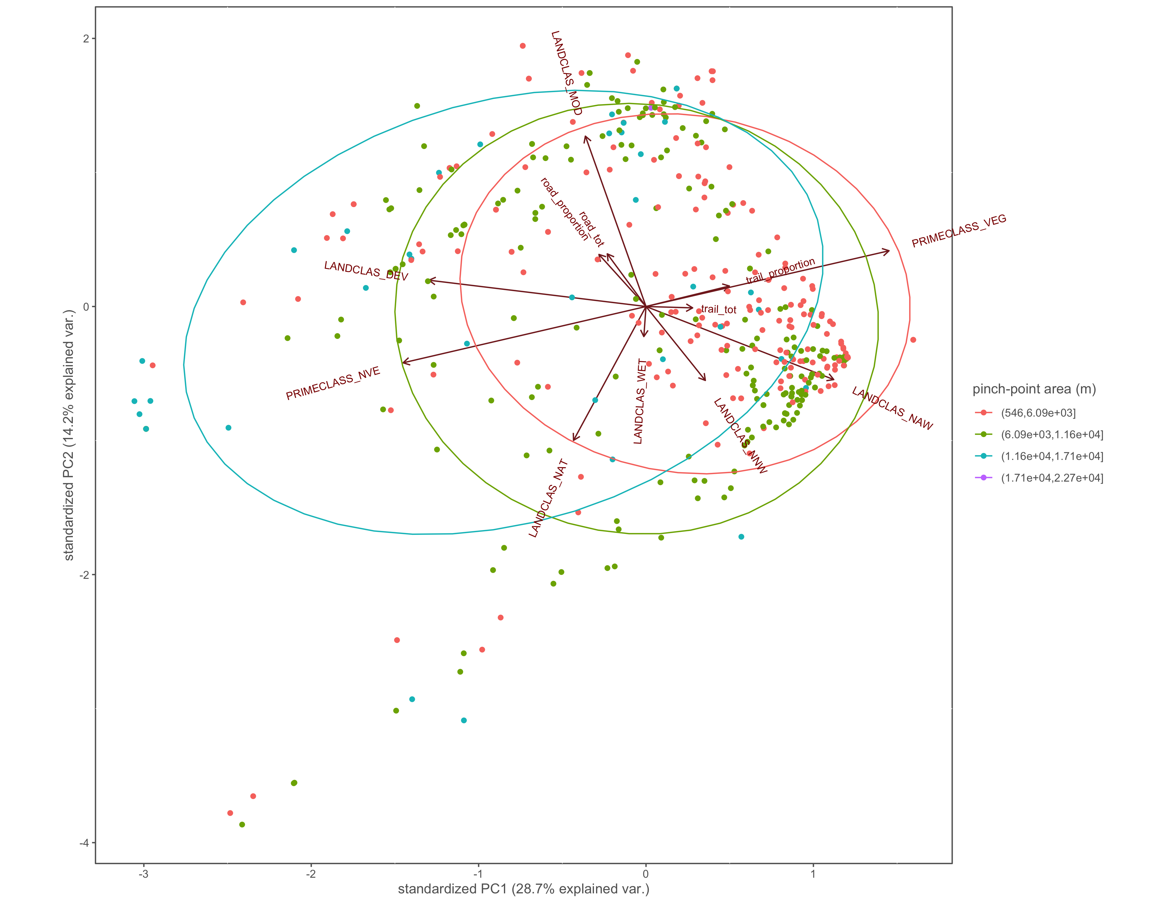
Figure 4.21: PCA biplot with pinch-points grouped by the pinch-point polygon area
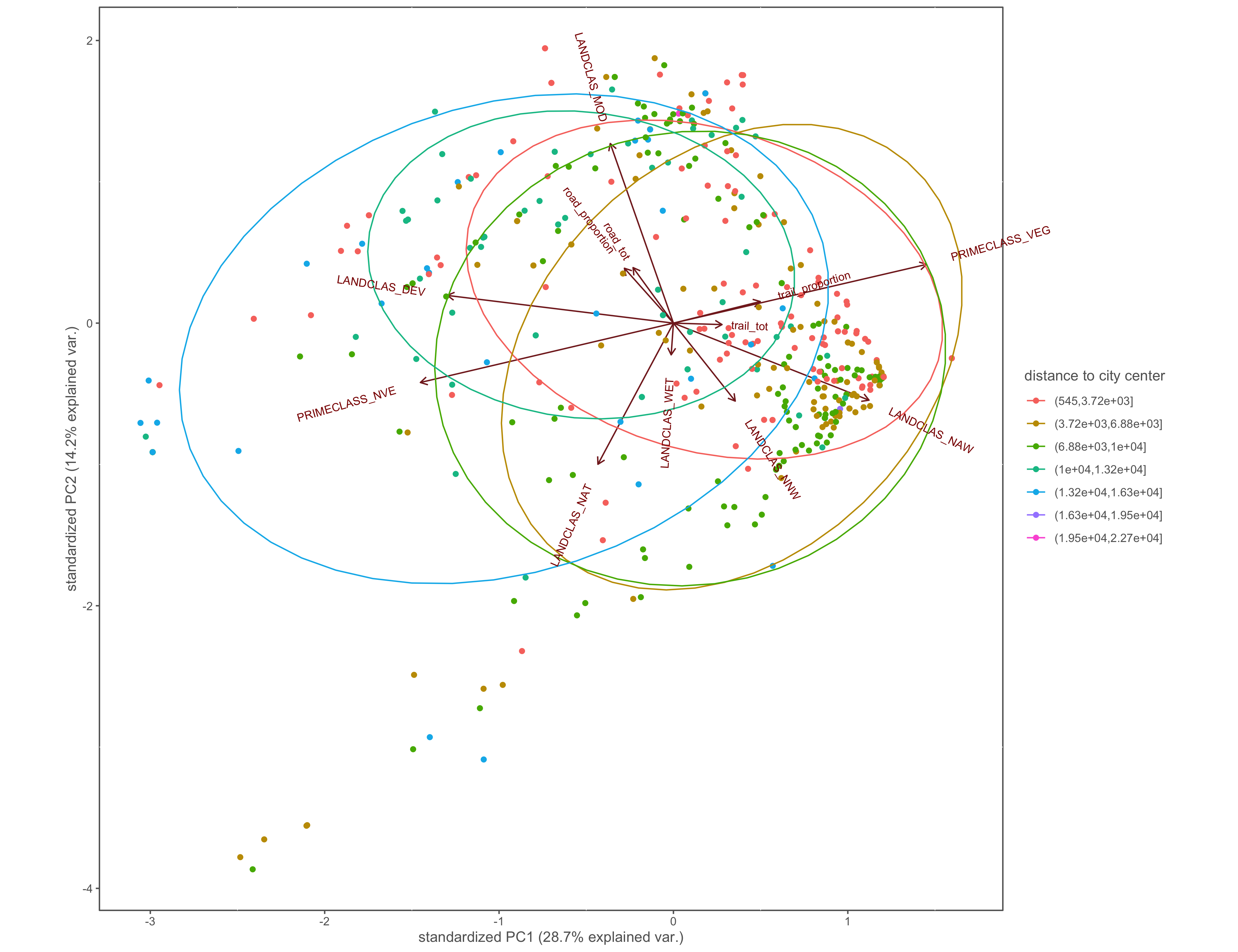
Figure 4.22: PCA biplot with pinch-points grouped by the distance to city center
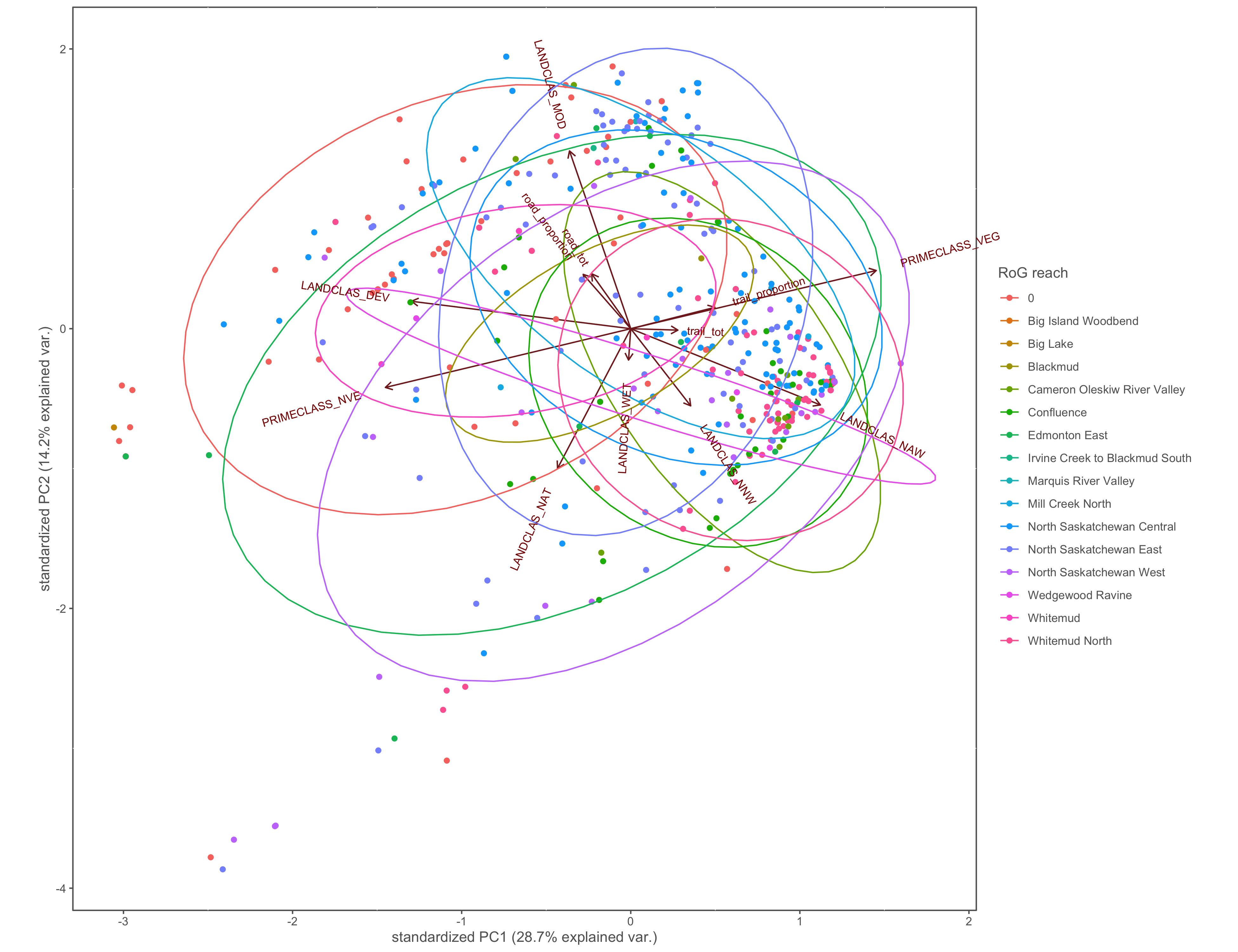
Figure 4.23: PCA biplot with pinch-points grouped by the RoG reach
hierarchical clustering of PCA
#hc<-hclust(dist(x.pca_2$loadings))

loadings = x.pca$loadings[]

    q = loadings[,1]
    y = loadings[,2]
    z = loadings[,3]


    hc = hclust(dist(cbind(q,y)), method = 'ward')

    png("4_output/PCA/interior_only/hclust_plot", width=1000, height=600)
    plot(hc, axes=F,xlab='', ylab='',sub ='', main='Clusters')
    rect.hclust(hc, k=3, border='red')
    dev.off()


# view clusters in biplot
x.pca2<-x.pca

# pct=paste0(colnames(x.pca2$x)," (",sprintf("%.1f",x.pca2$sdev/sum(x.pca2$sdev)*100),"%)")
p2=as.data.frame(x.pca2$x)


x.pca2$k=factor(cutree(hclust(dist(x), method='complete'  ),k=10))
ggbiplot(x.pca2,  ellipse=TRUE, groups=x.pca2$k)+
  labs(color="cluster")+
    custom_theme()
Figure 4.24: Hierarchical clusters of PCA variables