Section 24 Profile Analysis
Are there statistically significant differences between properties in different price quartiles?
Methodology
Since we are dealing with large sample sizes, such a test can be achieved with a One Way Multivariate Analysis of Variance Procedure (see MANOVA Section in the Introductory Theory Chapter).
Figure 24.1 shows why it is important to perform this test. The data is segmented according to (log) price quartile and the four mean co-ordinate vectors are plotted. (Each co-ordinate has been rescaled so that the units are comparable.) It is clear that the profiles of the four quartiles are very similar. Comparing the Highest and Lowest Price Quartiles, we see there are more multi-floor properties with higher condition and with views in the Highest Quartile. Otherwise there appear to be few differences.
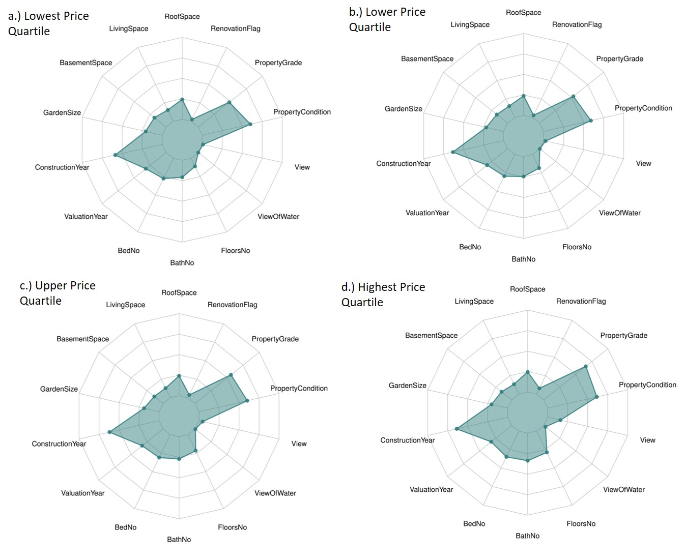
Figure 24.1: Looking for Relationships.
The following MANOVA strategy is recommended for Multivariate Comparisons of Treatments in Johnson, Wichern, and others (2014):
- Try to identify outliers
- Perform a multivariate test of hypothesis
- Calculate the Bonferroni simultaneous confidence intervals to identify components which differ significantly
Hypothesis Testing
\(H_{0}:\tau_{1}=\tau_{2}=\tau_{3}=\tau_{4}=0\). Lets perform a two sided test at the five percent significance level.
The test results below show that, for the data set exlusing outliers, the 0.453 value for Wilks Lambda is significant at the 0.1% level and hence \(H_{0}\) should be rejected.
##              Df   Wilks approx F num Df den Df    Pr(>F)
## quantile      3 0.45262   499.22     39  63430 < 2.2e-16 ***
## Residuals 21432
## ---
## Signif. codes:  0 '***' 0.001 '**' 0.01 '*' 0.05 '.' 0.1 ' ' 1
Following the recommendation in (Johnson, Wichern, and others (2014)), we repeat the test using the data with outliers.Again the value for Wilks Lambda of 0.453 is significant at the 0.1% level and hence \(H_{0}\) should be rejected.
##              Df   Wilks approx F num Df den Df    Pr(>F)
## quantile      3 0.45331   489.08     39  62278 < 2.2e-16 ***
## Residuals 21043
## ---
## Signif. codes:  0 '***' 0.001 '**' 0.01 '*' 0.05 '.' 0.1 ' ' 1
The Treatment effects and the width of the simultaneous Bonferroni confidence intervals (\(\alpha=0.05\))are given below. Due to the c5000 observations in each quantile the confidence intervals are very narrow and even small differences in treatment effects are significant.
| Base | Base->Q2 | Base->Q3 | Base->Q4 | BF Range | |
|---|---|---|---|---|---|
| sqft_above | 1316.20 | 241.64 | 440.82 | 1221.18 | 84.21 |
| RenovationFlag | 1.03 | 0.00 | 0.01 | 0.05 | 0.00 |
| grade | 6.81 | 0.49 | 0.90 | 2.04 | 0.00 |
| condition | 3.41 | -0.05 | -0.01 | 0.05 | 0.00 |
| View | 0.04 | 0.06 | 0.14 | 0.59 | 0.00 |
| WaterfrontView | 0.00 | 0.00 | 0.00 | 0.02 | 0.00 |
| NumberOfFloors | 1.28 | 0.18 | 0.26 | 0.44 | 0.00 |
| NumberOfBedrooms | 3.03 | 0.19 | 0.38 | 0.79 | 0.00 |
| NumberOfBathrooms | 1.66 | 0.30 | 0.51 | 1.01 | 0.00 |
| SaleYear | 2014.31 | 0.01 | 0.01 | 0.01 | 0.00 |
| ConstructionYear | 1967.35 | 5.60 | 3.83 | 5.54 | 0.15 |
| sqft_lot | 10501.79 | 2274.49 | 5447.66 | 10861.44 | 300962.16 |
| sqft_living | 1467.71 | 314.45 | 616.93 | 1534.64 | 91.02 |
Conclusion
We reject the Null at the 5% level, both with and without outliers, using the Wilks Lambda statistic. We conclude that there are statistically significant differences in the data between the mean vectors of the top, middle, lower and bottom price quartiles.
References
Johnson, Richard Arnold, Dean W Wichern, and others. 2014. Applied Multivariate Statistical Analysis. Vol. 4. Prentice-Hall New Jersey.