Section 26 Correlation Analysis
Does the enriched data-set contain new information or is there significant overlap with the original data?
Methodology
I will use Canonical Correlation Analysis to measure the degree of overlap between the two data sets (see Canonical Correlation Analysis for a theoretical introduction).
I expect significant overlap between the original and enriched data set. Variables in the original data set which do not represent geospatial information are indeed highly correlated with geospatial features. For example in figure 26.1, I used the sp package to aggregate 21,436 properties in 200m by 200m grids and then to plot the average construction year by grid. We see that the oldest properties are located in the north-west region and properties get progressively newer as we move east.
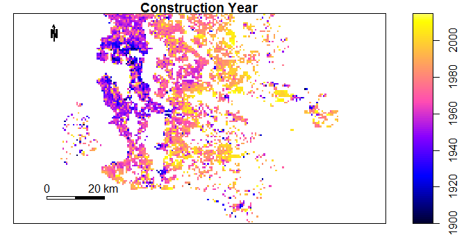
Figure 26.1: Number of Doctors or Dentists within 500m by Location
Model Fitting
I have modelled six Geospatial variables from the Enriched Data Set and 10 non-Geospatial variables from the Original Data set. The pair-wise correlations are shown below:
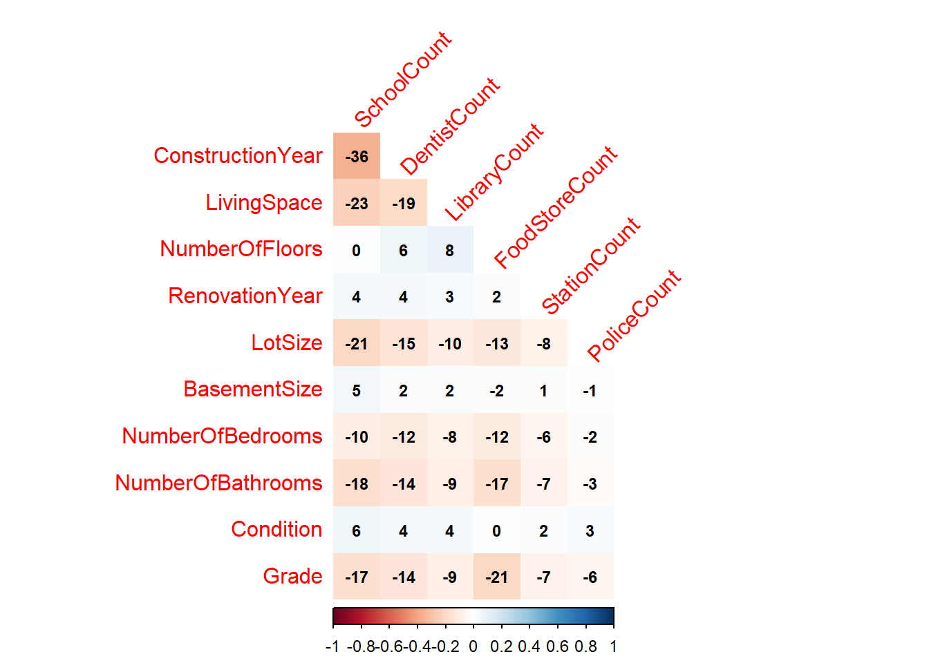
The correlations between the first six pairs of canonical variates are shown below. The Canonical Correlation between the first pair (V1, U1) is 57%, this is much higher than any entry in the correlation matrix above and shows the power of the canoncical co-ordinate transformation. There is clearly significant overlap between the information in each data-set.
| Corr1 | Corr2 | Corr3 | Corr4 | Corr5 | Corr6 |
|---|---|---|---|---|---|
| 0.57 | 0.15 | 0.13 | 0.06 | 0.05 | 0.02 |
Analysis
The correlation of each canonical variate with its respective data set is shown below. Variable V1 from the enriched data set is highly positively correlated with number of Schools, Dentists, Libraries and Food stores. V1 appears to measure Neighbourhood Services
U1 from the original data set is strongly negatively associated with Construction Year, Living Space, Lot Size, Number of Bedrooms. U1 appears to measure older, smaller properties.
The 57% correlation between V1 and U1 is likely explained by smaller, older properties being in highly urbanised areas near to lots of services. This can actually be visualised by comparing Figure 26.1 with the plots in the Enrichment Results Section.
| V1 | V2 | V3 | V4 | V5 | V6 | |
|---|---|---|---|---|---|---|
| SchoolCount | 0.91 | -0.03 | -0.40 | -0.08 | 0.09 | 0.03 |
| DentistCount | 0.78 | -0.03 | 0.24 | 0.21 | -0.10 | 0.52 |
| LibraryCount | 0.70 | -0.26 | 0.44 | -0.24 | 0.37 | -0.23 |
| FoodStoreCount | 0.64 | 0.71 | 0.16 | -0.25 | -0.05 | 0.05 |
| StationCount | 0.36 | 0.05 | 0.05 | 0.61 | -0.37 | -0.59 |
| PoliceCount | 0.12 | 0.29 | -0.05 | 0.54 | 0.77 | 0.13 |
| U1 | U2 | U3 | U4 | U5 | U6 | |
|---|---|---|---|---|---|---|
| ConstructionYear | -0.66 | 0.01 | 0.26 | 0.32 | -0.19 | -0.22 |
| LivingSpace | -0.44 | -0.61 | 0.12 | -0.18 | 0.31 | 0.12 |
| NumberOfFloors | 0.08 | -0.18 | 0.69 | 0.17 | 0.21 | -0.19 |
| RenovationYear | 0.08 | -0.08 | 0.02 | 0.27 | 0.11 | -0.17 |
| LotSize | -0.35 | -0.11 | 0.56 | -0.33 | -0.13 | -0.23 |
| BasementSize | 0.07 | -0.36 | -0.31 | 0.09 | -0.07 | 0.07 |
| NumberOfBedrooms | -0.23 | -0.28 | -0.26 | -0.25 | 0.53 | -0.54 |
| NumberOfBathrooms | -0.32 | -0.51 | 0.23 | 0.10 | 0.30 | -0.20 |
| Condition | 0.09 | -0.22 | -0.19 | 0.39 | 0.49 | 0.19 |
| Grade | -0.32 | -0.85 | 0.15 | -0.03 | -0.08 | -0.07 |
Conclusions
There is significant overlap between the Original Data set and the Original Data set. The value for the first canonical correlation was 57%. Even though it does not appear possible at first glance, variables such as Construction Year are associated with geospatial features. It is these geospatial patterns which generate the large canonical correlation values with the enriched data set.