Section 17 Data Source
The original data can be found on my GitHub site (Source Data). The data comprises a table with 21613 rows (one per property sale) and 19 columns of explanatory variables. Descriptions of each data column is shown below. The fields containing categorical data as opposed to numeric (discrete or continuous) are also identified. The absence of information for a particular property, in a particular field was encoded with a blank.
| Field Name | Data Type | Data Description |
|---|---|---|
| ID | Continuous Numeric | Unique Property Identifier |
| Date | Continuous Numeric | Date of Sale |
| Price | Continuous Numeric | Property Sale Price in USD |
| Bedrooms | Dicrete Numeric | Number of Bedrooms |
| Bathrooms | Dicrete Numeric | Number of Bathrooms |
| sqft_living | Continuous Numeric | Size of the Living Space in square feet |
| sqft_lot | Continuous Numeric | Total Size of the property in square feet |
| floors | Dicrete Numeric | Number of Floors in Property |
| waterfront | Categoric | 1=Waterfront View, 0=No Waterfront View |
| view | Categoric | Number of Sides of Property with View |
| condition | Categoric | Property Condition (1=Poor Condition 5= Excellent Condition) |
| grade | Categoric | Property Condition (1=Poor, 13= Excellent) |
| sqft_above | Continuous Numeric | Size of Upstairs Floors in square feet |
| sqft_basement | Continuous Numeric | Size of Basement in square feet |
| yr_built | Continuous Numeric | Construction Year |
| yr_renovated | Continuous Numeric | Year Property Renovated |
| zipcode | Categoric | Postal Code |
| lat | Continuous Numeric | Property Latitute |
| long | Continuous Numeric | Property Longitude |
Exploratory Analysis
For large, multivariate data sets it takes more time to search through and explore a data set. The plots below allow a quick inspection of the original data-set.
Whilst Visual inspection of the data table is tedious and unreliable, through sorting property ID’s, I was able to identify that a small number of properties appear multiple times in the data. This comes about due to a single property being sold more than once during within the data collection period. For my analysis, I chose to retain only the most recent transactional record for properties with multiple appearances. This process reduced the size of the data-table from 21613 to 21436 rows.
In figure 17.1, we that the largest 6% of all sale transactions by number, account for 18% of the total transactional value in the data. Furthermore, as can be seen this group of properties outlies the other property values.
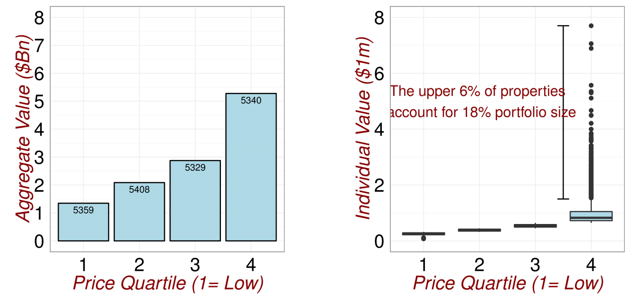
Figure 17.1: Revisiting the Data 1.
In figure 17.2, we see a large spread in the sizes of living spaces and a significant portion of properties without basements. In the lot size chart, we see again a large spread of sizes with a significant upper tail.
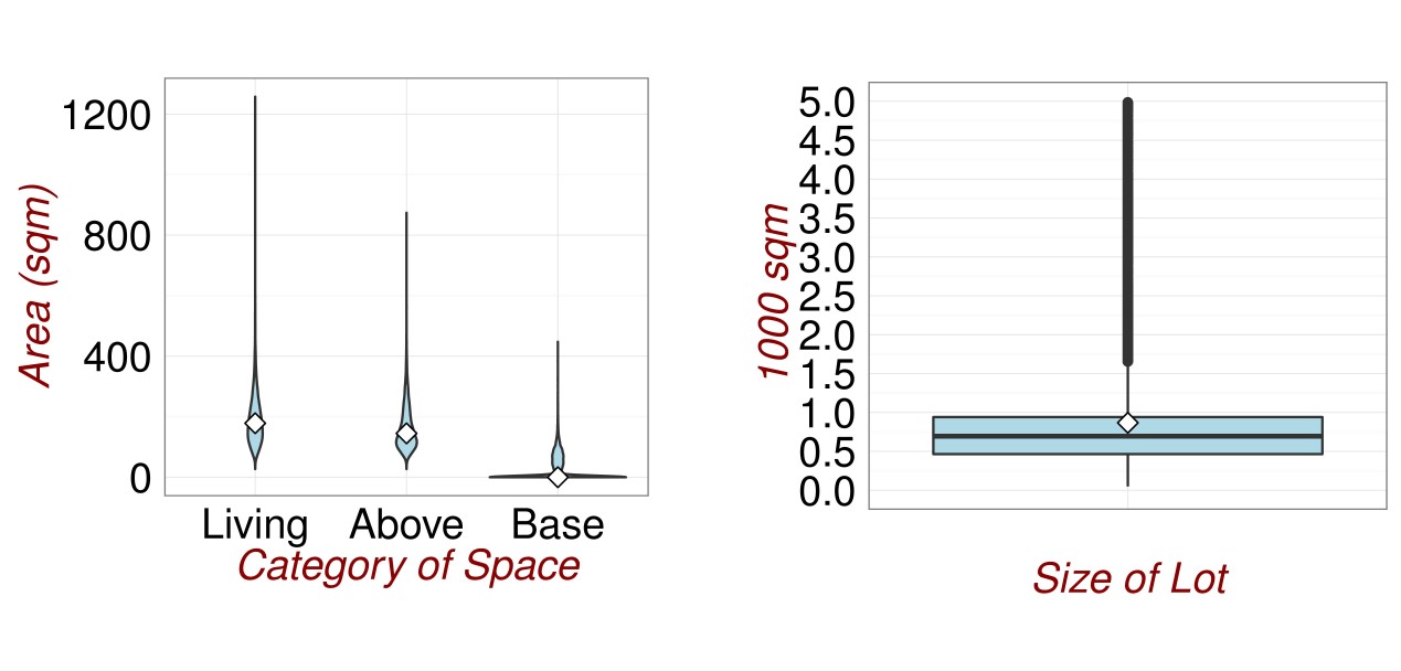
Figure 17.2: Revisiting the Data 2.
In figure 17.3, we see that the modal number of bedrooms is three and the modal number of bathrooms is 2. There are 13 and 85 properties with no bedrooms or no bathrooms respectively. These are understood to be data entry errors are are excluded from the analysis data sets. There is also one mid-value property in the data with 33 bedrooms, this should also be excluded as an error.
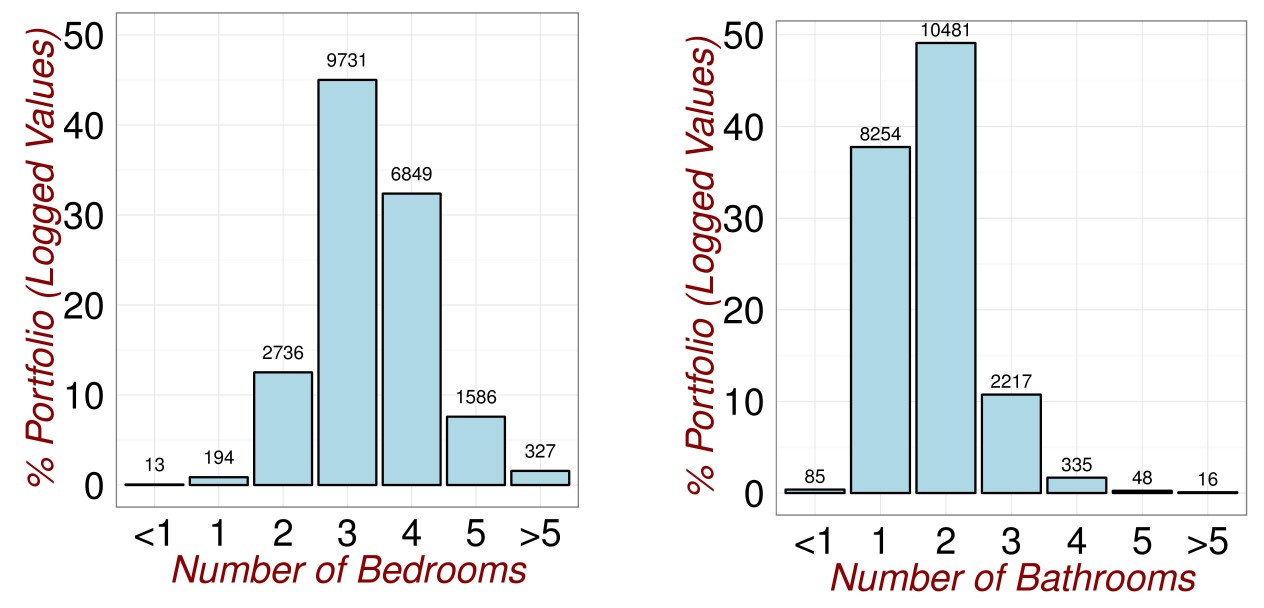
Figure 17.3: Revisiting the Data 3.
In figure 17.4, we see that the vast majority of the properties in the data-set do not have a waterfront view. This is surprising given the presence of significant lakes near to Seattle. We do see in figure 17.5, that a significant minority of properties do have a general view. It is possible that the low number of waterfront view properties is due to a very restrictive criteria set being applied (eg. property must be next to water for a waterfront view flag). The vast majority of the properties in the data are either single storey appartments or bungalows (10559) or two storey maisonettes (8209).
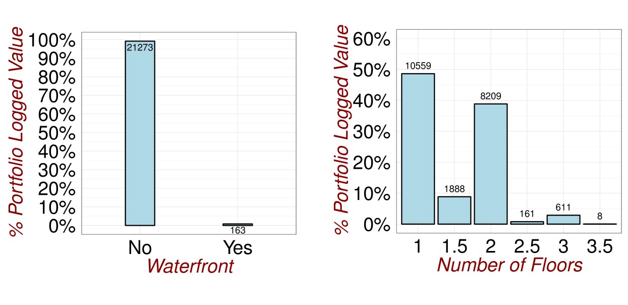
Figure 17.4: Revisiting the Data 4.
In figure 17.5, we see that a significant minority of the properties in the data-set (approx 10%) have a view on at least one side There are only 193 properties in the data-set in poor condition (ie. condition less than 2). Visual inspection of these records, shows that they were built in the early 20th century and may have become dilapidated.
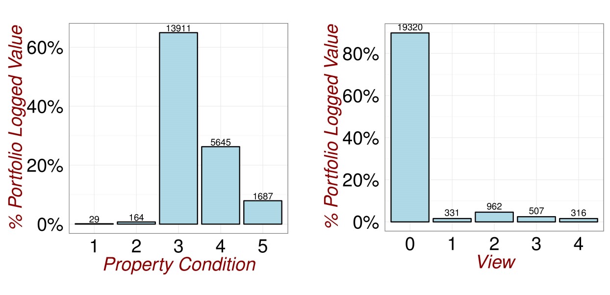
Figure 17.5: Revisiting the Data 5.
In figure 17.6, we see that the vast majority of properties were built in late 20th century and early 21st century. The earliest construction date in the data is 1900.The grade metric is another measure of property condition. As it has a wider range of values than “condition”, it looks like a better differentiator of properties in good and bad states of repair.
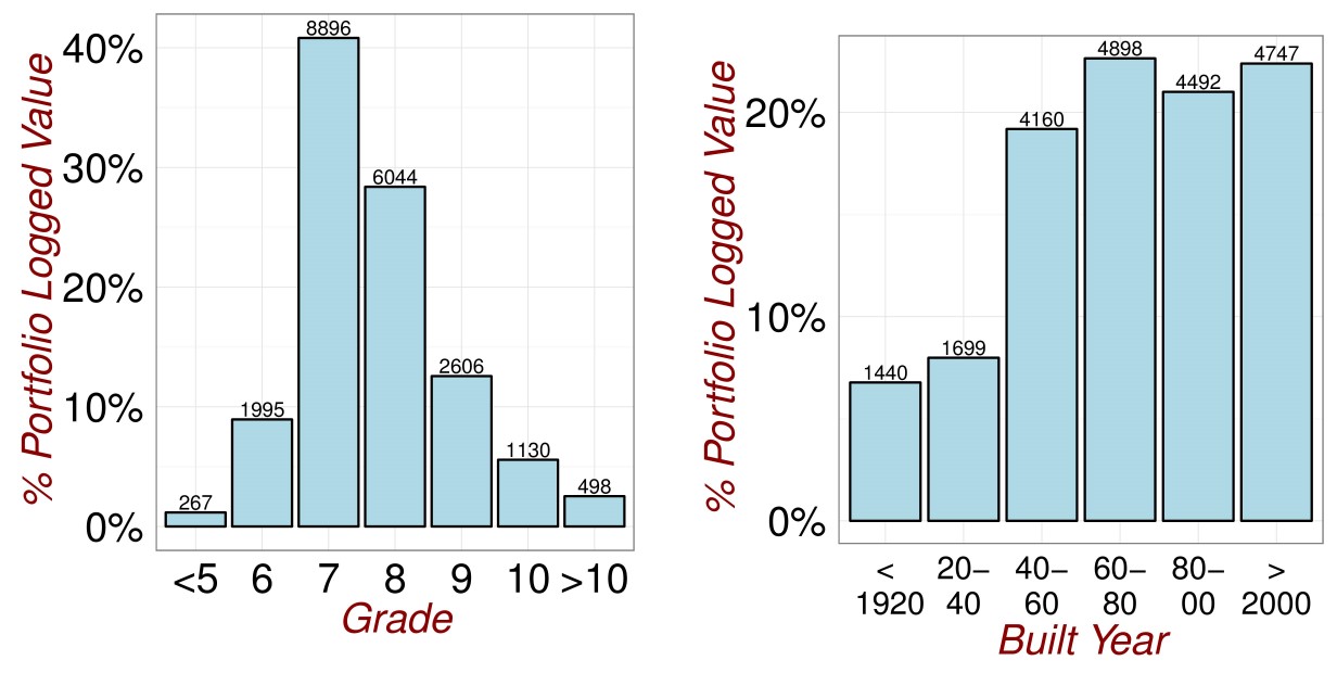
Figure 17.6: Revisiting the Data 6.