Section 18 Outliers and Errors
Multivariate Analysis
Powerful statistical techniques exist for detecting outliers in data generated by Multivariate normal distributions. Individual variables, when standardised, should follow the \(t_{n-1}\) distribution. The generalised distance \((x_{j}-\overline{x})^´S^{-1}(x_{j}-\overline{x})\) of each vector of observations \(\underset{(p \times 1)}{x_{j}}\) from the sample mean \(\overline{x}\) is approximately \(\chi_{p-1}^2\) distributed. This means that, in addition to univariate and bivariate scatter plots, we can numerically identify outliers as points corresponding to very low or very high significance levels (see Johnson, Wichern, and others (2014), Chapter 4, page 189).
By transforming the data first to standardised co-ordinates and then secondly to a principal component decomposition, I aimed to achieve approximate multivariate normality. I used the prcomp function in the stats package to obtain the principal components via a singular value decomposition. The first five principal components account for 80% of the Sample Variation in the data. As a check I have plotted the eigenvalues of the Sample Covariance Matrix in fig 18.1 below. The steep slope in this Scree plot is consistent with the Variance in the data being captured in a few coordinates:
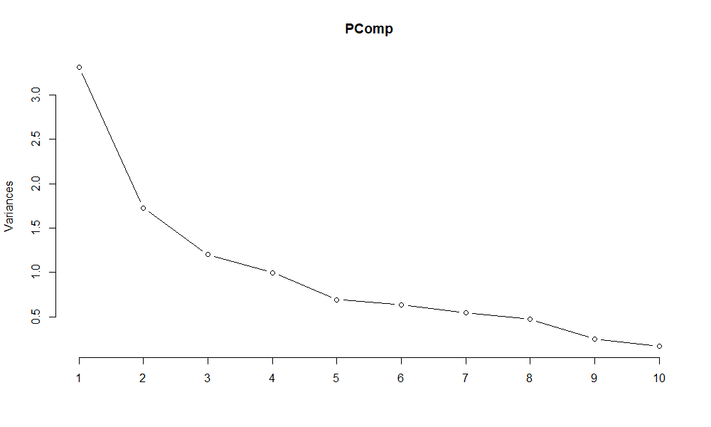
Figure 18.1: The eigenvalues of the 10 eigenvectors of the Sample Covariance Matrix are plotted.
The co-ordinates of the first 5 eigenvectors are shown in the summary table below. The first principal component (PC1) has positive components for almost all variables and places most weight on the number of bathrooms, the size of the living space, the price and the number of bedrooms. I interpret this principal component as a Market Index, measuring the base-line value of a property.
The second principal component (PC2) contrasts properties with scarce features in the data versus those with common features. High Property price, Condition, View or Waterfront are given large negative weight. Year Built and Floors have large positive weight. In this manner I interpret the second Principal Component as being a Scarcity/Uniqueness Index.
##                     PC1         PC2         PC3         PC4         PC5
## price        0.39474247 -0.32053152  0.01278184  0.05285835 -0.02822482
## bedrooms     0.33303751 -0.03437237  0.46408937  0.11463923  0.41251208
## bathrooms    0.48501509  0.09713638  0.11245838  0.04360269 -0.08736986
## sqft_living  0.48915976 -0.09806734  0.19258957 -0.04167929  0.09784782
## sqft_lot     0.08854103 -0.07595944  0.02822446 -0.97340504 -0.08146923
## floors       0.32522475  0.32827107 -0.20513390  0.11869523 -0.48638212
## waterfront   0.11427927 -0.39887998 -0.54652581  0.08931311 -0.06040434
## view         0.19703882 -0.46757283 -0.36367749  0.00819657  0.11018643
## condition   -0.10582765 -0.41352301  0.46447260  0.09074425 -0.71644655
## yr_built     0.28644948  0.46342508 -0.21250164 -0.05040852 -0.19884482
The bivariate scatter plots of the first five principal components are shown in Figure 18.2. By inspection of the many scattered points towards the top of the first row of charts, it is clear many properties have unusually high values for PC1. This is consistent with the upper-tail of high priced properties in figure 17.1 and I flagged all points with PC1 values above 10.5 as outliers.
In the second row of charts in Figure 18.2, there is a distinct cluster of points away from the main data cloud. This cluster of points is characterised by very low values for the Second Principal Component (PC2). I flagged all points with PC2 values below -6 as outliers, treating very high values for the “uniqueness” index similarly to very values for the “Market” Index PC1.
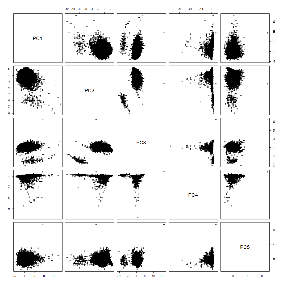
Figure 18.2: Bivariate plots of the PCA coordinate values. The distinct groups visible in all plots involving Principal Component 3 are due to discreteness in the data.
The procedure above removed 151 outliers points. Correspondingly, the bivariate scatter plots in figure 18.3 begin to resemble the smooth ellipses expected of Multivariate Normal Data.
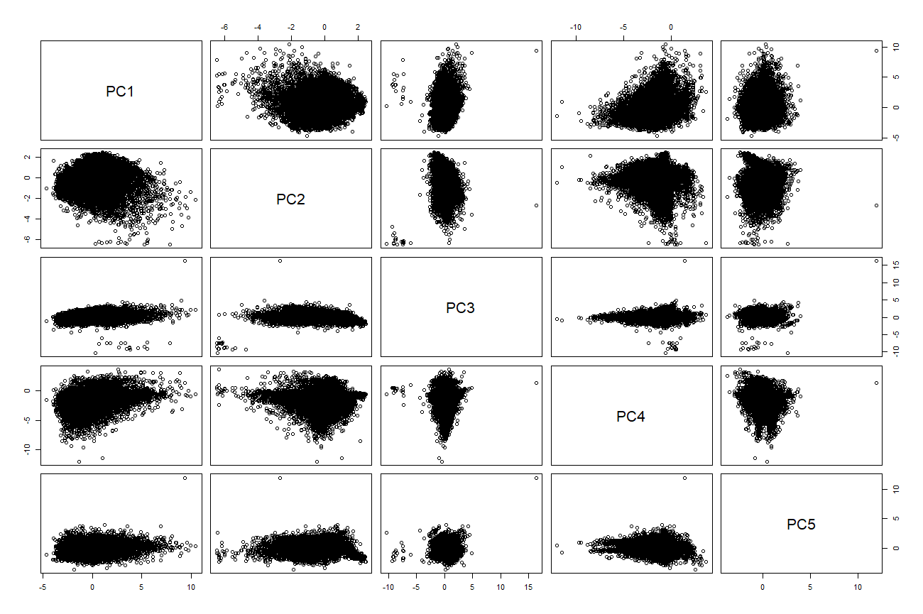
Figure 18.3: Bivariate plots of the PCA coordinate values with outliers removed.
If the multivariate normal assumption were appropriate and p=10, we would expect 5% of observations to have a generalised distance above 16.92. In fact in this data set 16% of observations lie above this.
We begin to understand why this has occurred by applying a Clustering Algorithm. The scatter plots in Figure 18.4 were generated using using the mcclust package in R to fit a Mixture of Normal Distributions . The Bayesian Information Criteria Value is significantly higher for a mixture of three (Equal Covariance) Multivariate Normal Distributions than for a single distribution.It is this heterogeneity in the data which makes the scatter plots in Figure 18.3 more disparate than otherwise.
Since according to Figure 18.4, outliers would still lie far from the centre of the data cloud, I used the 1% critical value of the \(\chi_{9}^2\) distribution to flag the outermost data points as outliers. In this manner 563 additional data points (2.6% data) were flagged as outlying.
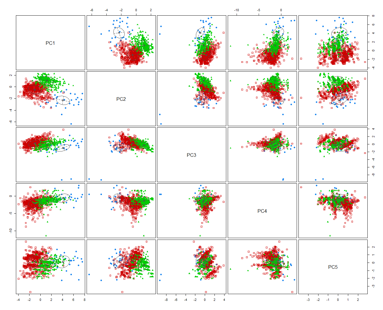
Figure 18.4: Bivariate plots of the PCA coordinate values with outliers removed.
References
Johnson, Richard Arnold, Dean W Wichern, and others. 2014. Applied Multivariate Statistical Analysis. Vol. 4. Prentice-Hall New Jersey.