Section 7 Classical Linear Regression

Analytical Properties

A regression function is a conditional expectation. The expectation is calculated for one variable \(Y\), the response, conditional on the values for the other “explanatory” variables \(Z_{1},Z_{2},...,Z_{r}\). It need not be linear but always predicts \(Y\) with smallest MSE (ref Rao et al. (1973)). The regression function is written \(E[Y \vert Z_{1},Z_{2},...,Z_{r}]\).

We can motivate the form of the classical linear regression model with reference to the Multivariate Normal Distribution (ref Johnson, Wichern, and others (2014), page 404, eqn. 7.51):

Example 7.1 (Regression Function for Multivariate Random variables) Let \(Y\) and \(Z_{1},Z_{2},...,Z_{r}\) be generated by a Multivariate Normal Distribution, ie.:

\[\begin{bmatrix}Y\\ Z_{1}\\...\\Z_{r}\end{bmatrix} \sim \mathcal{N}_{r+1}(\mu,\Sigma)\]

We can then infer the conditional distribution of \(Y\) given \(Z_{1},Z_{2},...,Z_{r}\). Using the notation of definition 5.3:

\[Y_{\vert Z_{1},Z_{2},...,Z_{r}} \sim \mathcal{N}_{1}(\mu_{Y}+\sigma_{XY}^{´}\sigma_{ZZ}^{-1}(Z-\mu_{Z}),\sigma_{YY}-\sigma_{ZY}^{´}\sigma_{ZZ}\sigma_{ZY})\]

We can then identify the regression function as a linear function of the vector of explanatory variables \(Z\) plus a constant term:

\[E[Y \vert Z_{1},Z_{2},...,Z_{r}]=\mu_{Y}+\sigma_{XY}^{´}\sigma_{ZZ}^{-1}(Z-\mu_{Z})\]

By making the following definitions:

\[\begin{align} b_{Z} &:= \Sigma_{ZZ}^{-1}\sigma_{ZY}\\ b_{0} &:= \mu_{Y}-b_{Z}^{´}\mu_{Z} \end{align}\]

We can write the regression function in the following form:

\[E[Y \vert Z_{1},Z_{2},...,Z_{r}]=b_{0}+b_{Z}^´Z\]

\(\square\)

In the classical linear regression model, we call the linear predictor a mean effect.The response \(Y\) is generated from the mean effect by adding an error term (see Johnson, Wichern, and others (2014), page 362, eqn. 7.3).

Definition 7.1 (Classical Linear Regression Model) Let \(Y\) be a univariate response variable whose relationship with r predictor variables \(Z_{1},Z_{2},...,Z_{r}\) is under investigation. The classical Linear Regression Model is:

\[\begin{align} Y &= \beta_{0}+\beta_{1}Z_{1}+\beta_{2}Z_{2},...+\beta_{r}Z_{r}+\epsilon \\ [Response] &= [Mean]+[Error] \end{align}\]

The following additional assumptions are made. For a Random Sample of size n, we assume:

The error term has zero expectation: \[E[\underset{(n \times 1)}{\epsilon}]=\underset{(n \times 1)}{0}\]

The individual components of the error vector have equal variance and are mutually uncorrelated:

\[\underset{(n \times n)}{Cov(\epsilon)}=\sigma^2\underset{(n \times n)}{I}\]

The error vector is generated by a multivariate normal distribution:

\[\underset{(n \times 1)}{\epsilon} \sim \mathcal{N}_{n}(0,\sigma^2I)\]

\(\square\)

When fitting classical linear models, it is important to remember that the explanatory variables \(Z\) are considered fixed but the parameter values \([\beta_{0},\beta_{1},..,\beta_{r}]\) need to be determined .

The geometrical picture of a Classical Linear Regression model is as follows (see Johnson, Wichern, and others (2014), page 367):

Definition 7.2 (Geometrical Picture of Linear Regression) The expected value of the response vector is:

\[E[Y]=X\beta=\begin{bmatrix}1 & Z_{11} & Z_{12} & ...& Z_{1r}\\1& Z_{21} & Z_{22} &\dots & Z_{2r}\\\vdots&\vdots&\vdots&\ddots&\vdots\\1 & Z_{n1} & Z_{n2} &\dots&Z_{nr}\end{bmatrix} \begin{bmatrix}\beta_{0}\\\beta_{1}\\\vdots\\\beta_{r}\end{bmatrix}\]

This can be re-written as a sum of the columns of Z:

\[E[Y]=\beta_{0}\underset{(n \times 1)}{1}+ \beta_{1}\underset{(n \times 1)}{Z_{1}}+...\beta_{r}\underset{(n \times 1)}{Z_{r}}\]

Thus the linear regression model states that the mean vector lies in a hyperplane spanned by the r+1 measurement vectors. These vectors are fixed by the measurement data and model fitting corresponds to finding the parameter values \([\beta_{0},\beta_{1},..,\beta_{r}]\) which minimise the Mean Square Error of the sample data.

The hyperplane is known as the model plane.

\(\square\)

Model Fitting

Estimating the best linear predictor (aka. the mean effect) for a Classical Linear Regression model can be achieved with ordinary least squares (OLS). Geometrically the OLS estimation procedure finds sample estimates for the parameter values \([\beta_{0},\beta_{1},..,\beta_{r}]\) which place the response vector \(y\) and a vector in the model plane as close together as possible. This corresponds to decomposing the response vector \(y\) in terms of a projection onto the model plane (aka. the prediction vector) and a vector of residuals orthogonal to the model plane (aka. the residual vector)

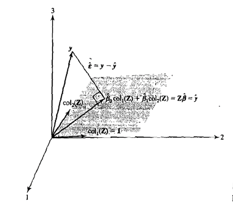
Figure 7.1: A representation of OLS model fitting with three observations (\(n=3\)) of one explanatory variable (\(col_{2}(Z)\)). Reproduced from Johnson, Wichern, and others (2014), Figure 7.1.

The following analytical result for OLS estimates can be derived (see Johnson, Wichern, and others (2014), page 364, eqn. 7.1):

Proposition 7.1 (OLS Estimates of Linear Regression Model) The r+1 dimensional vector of sample estimates for the parameter values \(\beta=[\beta_{0},\beta_{1},..,\beta_{r}]\) are denoted \(\widehat{\beta}=[b_{0},b_{1},..,b_{r}]\). The OLS estiamtes of \(\widehat{\beta}\):

\[\widehat{\beta}=(Z^´Z)^{-1}Z^´y\]

The n dimensional projection of the response vector onto the model plane is known as the prediction vector and denoted \(\widehat{y}\). The OLS estimate is:

\[\widehat{y}=Z(Z^´Z)^{-1}Z^´y\]

The n dimensional vector of differences between the responses \(y\) and the predictions \(\widehat{y}\) is known as the residual vector and denoted \(\widehat{\epsilon}\). The OLS estimate is:

\[\widehat{\epsilon}=(1-Z(Z^´Z)^{-1}Z^´)y\].

\(\square\)

The ability of the best linear predictor to explain variations in the response vector is estimated using the Coefficient of Determination (\(=\rho_{Y(Z)}^2\) see def. 5.3 ). (For proof see Johnson, Wichern, and others (2014), page 367, eqn. 7.9)

Proposition 7.2 (Measuring the Performance of Best Estimator) The orthogonality of \(\widehat{\epsilon}\) and \(\widehat{y}\) under OLS fitting allows the decomposition:

\[\begin{align} \sum_{i=1}^{n}(y_{i}-\overline{y})^2 &= \sum_{i=1}^{n}(\widehat{y_{i}}-\overline{y})^2 + \sum_{i=1}^{n}(y_{i}-\widehat{y_{i}})^2 \\ [Total Sum of Squares] &= [Regression Sum of Squares]+[Residual Sum of Squares] \end{align}\]

The coefficient of determination \(R^2\) is calculated as follows:

\[\begin{align} R^2 &= 1-\frac{\sum_{i=1}^{n}(y_{i}-\widehat{y_{i}})^2}{\sum_{i=1}^{n}(y_{i}-\overline{y})^2} \\ &= \frac{\sum_{i=1}^{n}(\widehat{y_{i}}-\overline{y})^2}{\sum_{i=1}^{n}(y_{i}-\overline{y})^2} \\ &= [Regression Sum of Squares]/[Total Sum of Squares] \end{align}\] \(\square\)

If the model assumptions in definition 7.1 are valid then the Sample Estimates of the model parameters have the following distributional properties (see Johnson, Wichern, and others (2014), page 404, page 370, section 7.4):

Proposition 7.3 (Sampling Properties of OLS Estimates) The parameter estimates \(\widehat{\beta}\) have the following properties:

\[\begin{align} E[\widehat{\beta}] &= \beta \\ Cov[\widehat{\beta}] &= \sigma^2(Z^´Z)^{-1} \\ \widehat{\beta} &\sim \mathcal{N}_{r+1}(\beta,\sigma^2(Z^´Z)^{-1}) \\ \end{align}\]

The sample estimates of the error term:

\[\begin{align} s^2 &:= \frac{\widehat{\epsilon}^´\widehat{\epsilon}}{n-(r+1)} \\ E[s^2] &= \sigma^2 \\ \widehat{\epsilon}^´\widehat{\epsilon} &\sim \sigma^2\chi_{n-r-1}^2 \end{align}\] \(\square\)

References

Rao, Calyampudi Radhakrishna, Calyampudi Radhakrishna Rao, Mathematischer Statistiker, Calyampudi Radhakrishna Rao, and Calyampudi Radhakrishna Rao. 1973. Linear Statistical Inference and Its Applications. Vol. 2. Wiley New York.

Johnson, Richard Arnold, Dean W Wichern, and others. 2014. Applied Multivariate Statistical Analysis. Vol. 4. Prentice-Hall New Jersey.