Section 27 Multivariate Regression Analysis
How accurately can we model property prices using a linear model?
Methodology
I am going to use a multiple linear regression model to model house prices. Please see the Linear Regression Section for an introduction to the technique.
I expect a significant proportion of the variance in property values to be explained by a Linear Model. This follows from the univariate plots in Figure 27.1. Each of these charts gives a bivariate scatter plot of Log Sale Price vs a single covariate from the Original Data set. Each scatter graph is overplotted with the line of best fit from a univariate regression model.
Visually each of the univariate plots appear consistent with the assumptions of the classical regression model. No trend is apparent in the residuals of the models: the lines of best fit bisect the data cloud evenly at a range of covariate values. The variance of the noise term is constant: the dispersion of points above and below the lines of best fit is approximately constant for all covariate values.(Independence of error terms is not checked.)
Large univariate \(SS_{reg}\) values are observed for Sqft_living, sqft_basement,Sqft_Above, Grade and Number of Bedrooms. These covariates individually explain a larger proportion of the variance in the log property sale price.
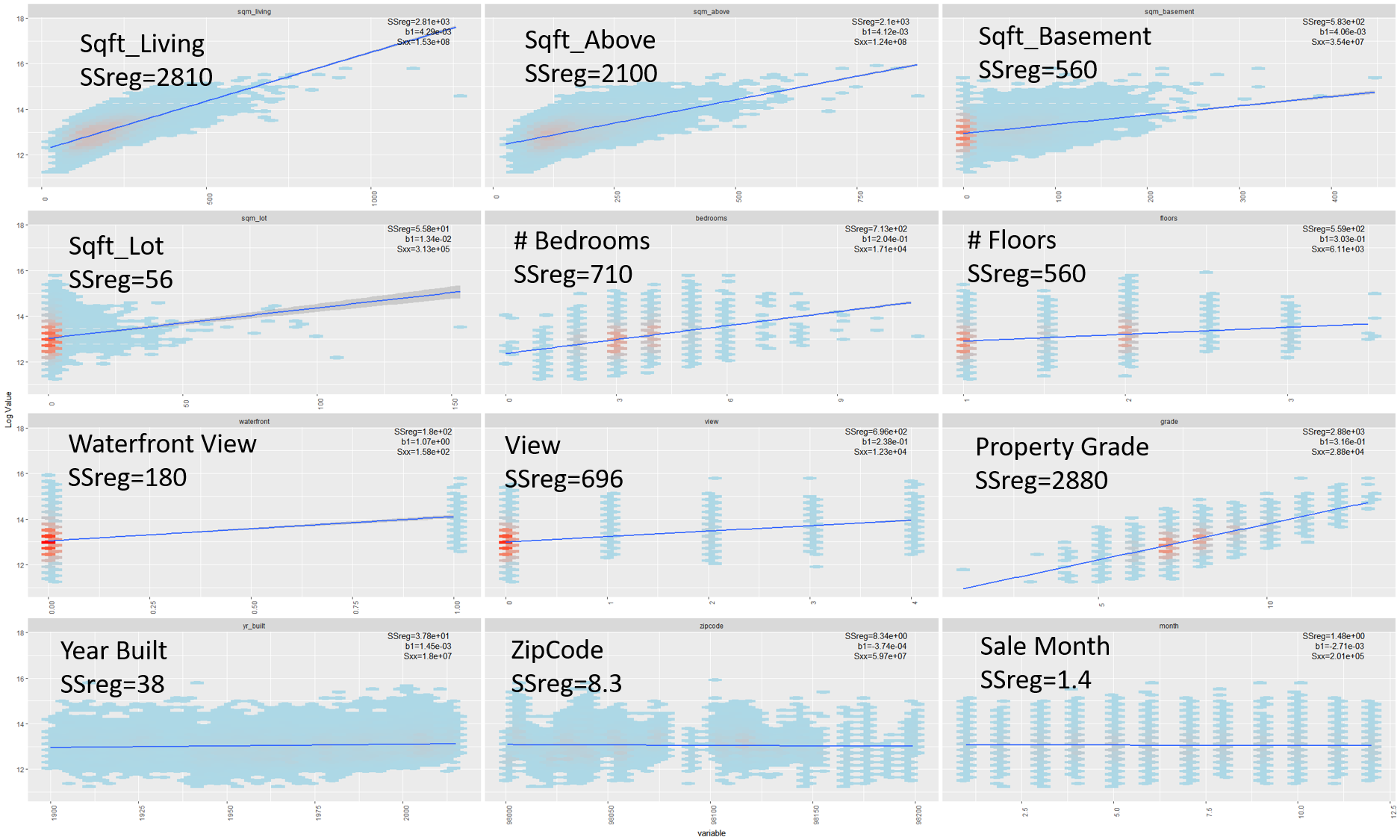
Figure 27.1: Linear Relations in the Original Data Set.
By contrast, I do not expect the variables from the Enriched Data Set to have significant explanatory power in a Multivariate Linear Regression Model. In Figure 27.2, I have repeated the univariate scatter plots using the Enriched Data set. These scatter plots have significantly lower \(SS_{reg}\) terms in comparison to those in Figure 27.1.
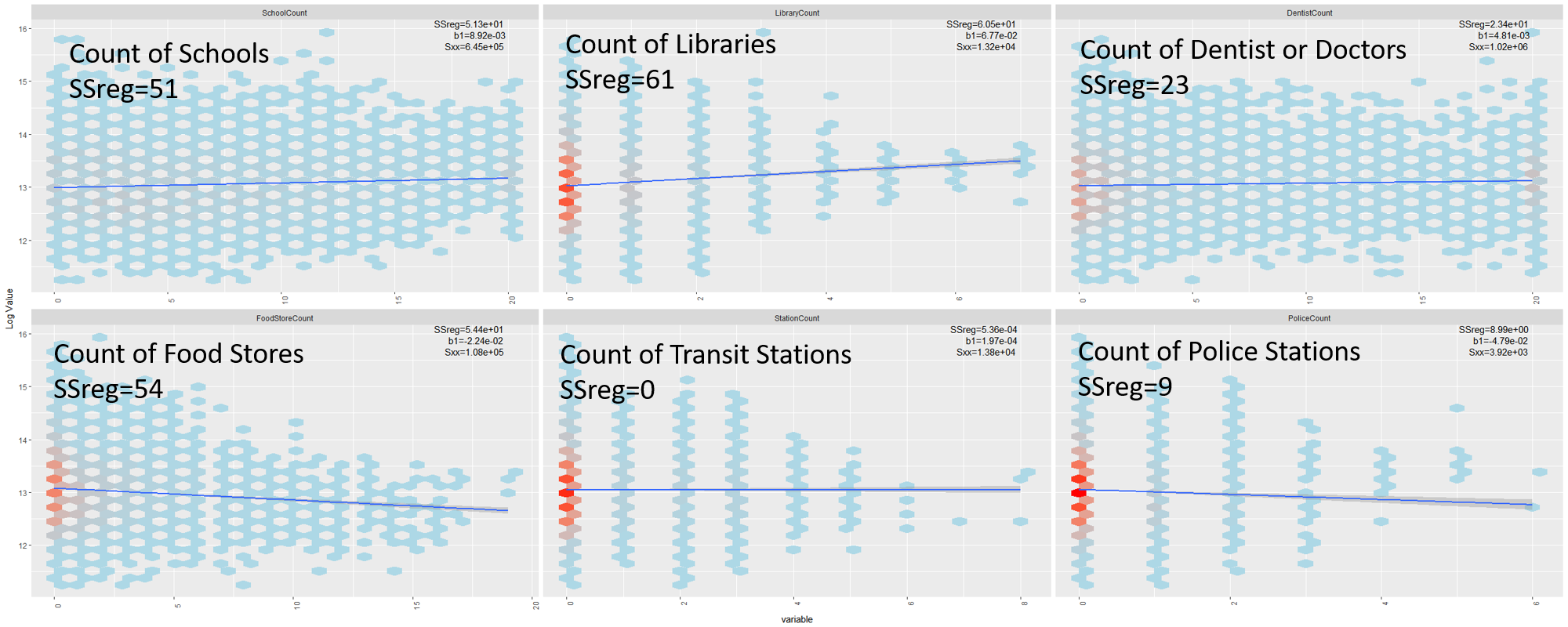
Figure 27.2: Linear Relations in the Enriched Data Set.
Model Fitting
To determine how accurately we can model property prices, I applied a step-wise Akaike fitting criterion from the MASS package. My starting model contained no covariates. I used the fully specified model, containing all variables in the data, to define an upper limit on the selection procedure.
library(MASS)

null<-lm(LogSalePrice ~
           1,data4)

full<-lm(LogSalePrice ~
           .,data4)

output<-step(null,scope=list(lower=null,upper=full),direction="both",scale=20)
The Akaike Criterion has a scale parameter which is used increase the penalty term for models with a large number of parameters. The results below show the impact of changing the scale parameter in the step-wise fitting procedure. The Scale Parameters were 100, 20, 10, 2, and 0.1 respectively for Models 1, 2, 3, 4, 5.
It is clear that reducing the penalty term leads to selecting models with more parameters. In all five models Grade, Living Space and Count of Schools are within the first four covariates to enter the model. This is consistent with their high \(SS_{reg}\) values in Figures 27.1 and 27.2. Furthermore, with the exception of Model 5, the signs of the parameters in all models are consistent with the slopes of the Univariate Lines of Best Fit in Figures 27.1 and 27.2.
Whilst the extra parameters in the models 4 and 5 do remain significant, they don’t however lead to large increases in the \(R^2\) value. The maximum \(R^2\) value is in the region of 68%.
| Model 1 | Model 2 | Model 3 | Model 4 | Model 5 | ||
|---|---|---|---|---|---|---|
| (Intercept) | 17.93*** | 17.00*** | 16.79*** | 16.63*** | 16.59*** | |
| (0.17) | (0.17) | (0.16) | (0.19) | (0.21) | ||
| Grade | 0.23*** | 0.22*** | 0.22*** | 0.21*** | 0.21*** | |
| (0.00) | (0.00) | (0.00) | (0.00) | (0.00) | ||
| ConstructionYear | -0.00*** | -0.00*** | -0.00*** | -0.00*** | -0.00*** | |
| (0.00) | (0.00) | (0.00) | (0.00) | (0.00) | ||
| LivingSpace | 0.00*** | 0.00*** | 0.00*** | 0.00*** | 0.00*** | |
| (0.00) | (0.00) | (0.00) | (0.00) | (0.00) | ||
| SchoolCount | 0.02*** | 0.02*** | 0.02*** | 0.02*** | 0.02*** | |
| (0.00) | (0.00) | (0.00) | (0.00) | (0.00) | ||
| View | 0.08*** | 0.06*** | 0.06*** | 0.06*** | ||
| (0.00) | (0.00) | (0.00) | (0.00) | |||
| WaterfrontView | 0.43*** | 0.43*** | 0.42*** | |||
| (0.03) | (0.03) | (0.03) | ||||
| FoodStoreCount | -0.02*** | -0.02*** | -0.02*** | |||
| (0.00) | (0.00) | (0.00) | ||||
| LibraryCount | 0.05*** | 0.04*** | 0.04*** | |||
| (0.00) | (0.00) | (0.00) | ||||
| Condition | 0.05*** | 0.05*** | ||||
| (0.00) | (0.00) | |||||
| NumberOfBathrooms | 0.06*** | 0.06*** | ||||
| (0.00) | (0.00) | |||||
| DentistCount | 0.00*** | 0.00*** | ||||
| (0.00) | (0.00) | |||||
| NumberOfBedrooms | -0.02*** | |||||
| (0.00) | ||||||
| PoliceCount | -0.04*** | |||||
| (0.00) | ||||||
| RenovationYear | 0.00*** | |||||
| (0.00) | ||||||
| LotSize | 0.00*** | |||||
| (0.00) | ||||||
| NumberOfFloors | 0.03*** | |||||
| (0.00) | ||||||
| R2 | 0.65 | 0.67 | 0.68 | 0.69 | 0.69 | |
| Adj. R2 | 0.65 | 0.67 | 0.68 | 0.69 | 0.69 | |
| Num. obs. | 21047 | 21047 | 21047 | 21047 | 21047 | |
| RMSE | 0.31 | 0.31 | 0.30 | 0.30 | 0.30 | |
| p < 0.001, p < 0.01, p < 0.05 | ||||||
Model Selection and Checking
I selected to check the consistency of Model 4 with the assumptions of the Classical Regression Model.
Given the large size of the data-set without outliers (21047 points), no points were found with high leverage or influence. The residual errors of the model should display no discernible trend and be consistent with white noise (ie. 95% of points within an interval of +/-1.96\(\sigma\)). Figure 27.3, shows the (standardised) residual errors of Model 4 plotted versus a number of Covariates. These plots are consistent with the classical regression assumptions.
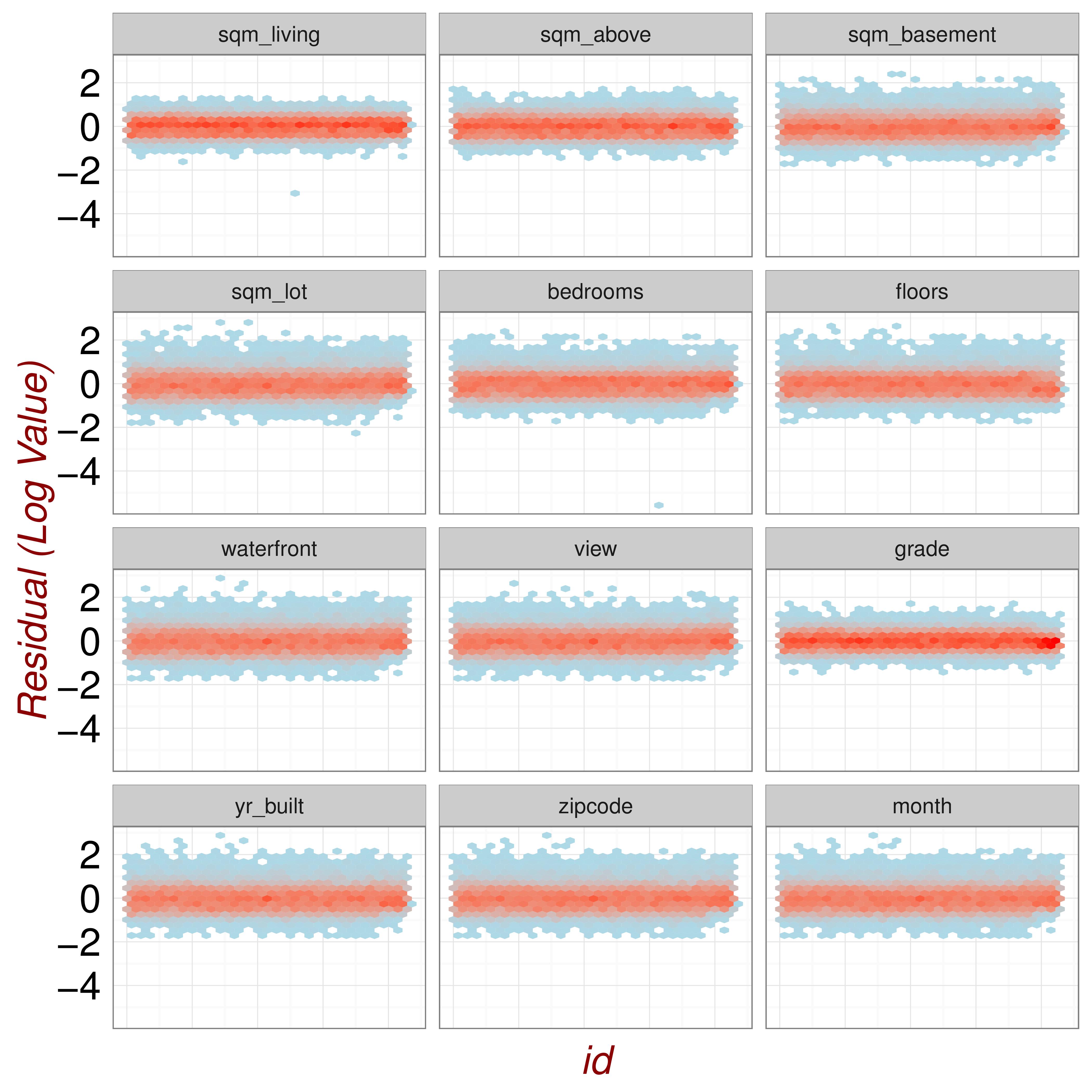
Figure 27.3: Residual Plots
In the Multivariate Regression model, the noise term is generated by a univariate normal distribution. Figure 27.4, gives quantile-quantile plots for the residuals of model 4 versus those of a normal distribution. The points closely fit a straight line, which is consistent with the model residuals being generated by a \(N(0,\sigma^2)\) distribution.
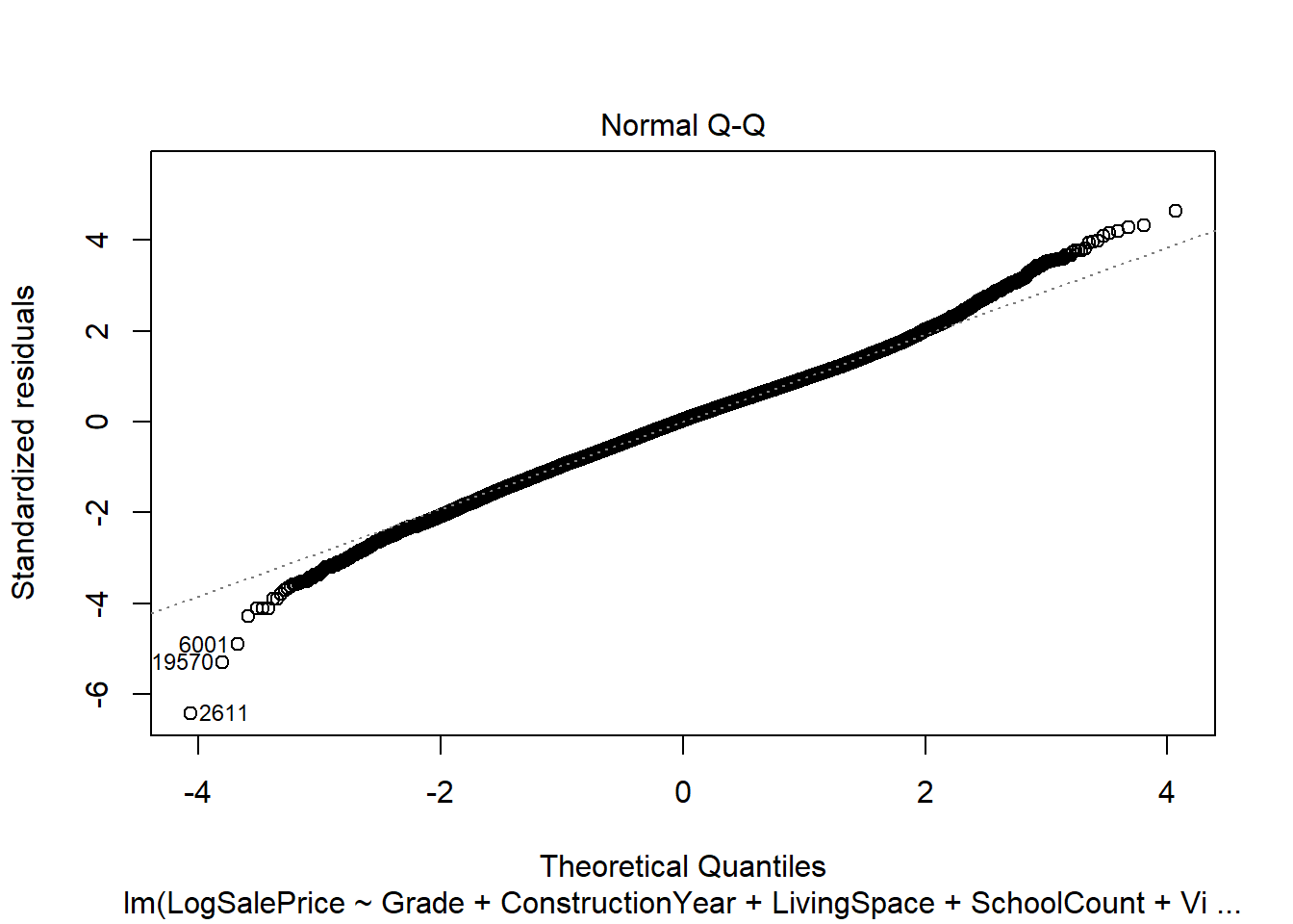
Figure 27.4: QQPlots
Conclusion
It is possible to fit a linear model to the Property Data Set and explain around 68% of the variation in (Logged) Property Prices. Furthermore such a model is compatible with the assumptions of a Multiple Linear Regression Model.