Section 25 Factor Analysis
Is it possible to describe a Property data set with a few variables? Do these variables have sensible interpretations?
Methodology
I will use Orthogonal Factor Analysis, to investigate whether the original data is consistent with a lower dimensional description (see Factor Analysis for theoretical introduction).
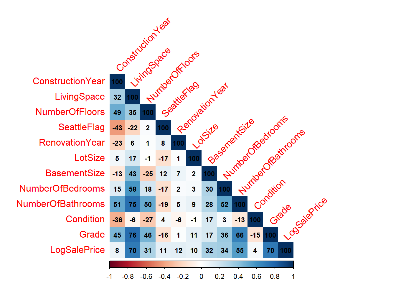
Factor Analysis is designed to group variables with high pairwise correlations. In the data, Number of Bathrooms, Grade, Living Space, Number of Bedrooms and LogSalePrice all have large pairwise correlations (see below). It is therefore compelling to perform a Factor Anaysis:
It is important to note that there is no clearly defined procedure for measuring the quality of a Factor Analysis (see Johnson, Wichern, and others (2014), Chapter 9, page 526 for further comments). Judging the success of a Factor Analysis depends on the subjective opinion of the investigator. Factor Anaylsis can have “Wow” factor by revealing insights that would otherwise be missed.
Model Fitting
I applied a Principal Component Solution to the Orthogonal Factor Model using the psych and nFactors packages in R. Prior to applying the Factor Model, I standardised all the variables to have zero mean and unit variance. I estimated the Principal Components using a Singular Value Decomposition Method. As is convention when seeking to improve the interpretability of Principal Components, I performed an orthogonal Varimax rotation.
The scree plot in Figure 25.1 indicated that five factors were an acceptable approximation to the data:
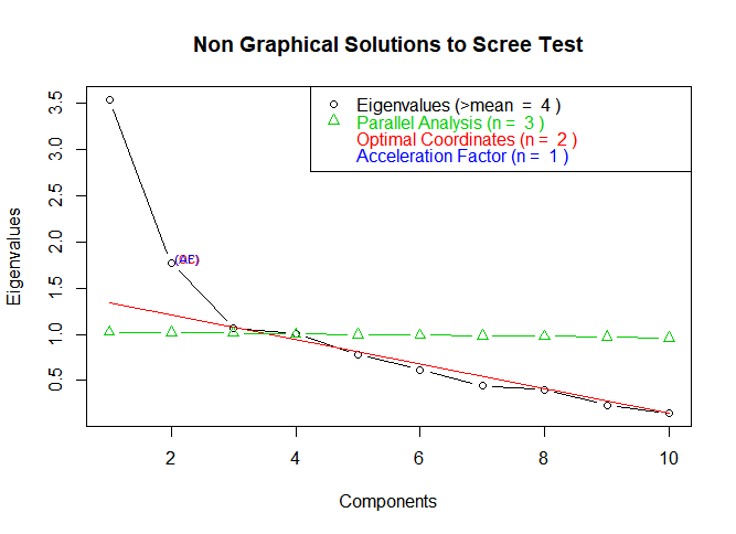
Figure 25.1: Number of Components in Factor Analysis
Results
The results of model fitting are shown below. The top block of results gives the co-ordinate representation of each of the five Orthogonal Factors (Column Headings RC1,..). The second block of results below gives the proportion of the total sample variance in the data explained by each Factor. The Factors have been ordered with decreasing eigenvalues.
Overall using Five Factors it is possible to explain 80% of the variation in the 10 variables (cf. Cumulative Var). This represents a good fit. A linear relationship with 5 Common Factors is able to explain 80% of the variation in 10 Variables with the remaining 20% assumed to be noise.
In the Orthogonal Factor Model (see Proposition 10.1, the “h2” column gives the %age of each variable’s variance attributable to the five Common Factors. Number of Bedrooms is the only variate for which the first Five Factors only explains less than 70% of the variance.
## Principal Components Analysis
## Call: principal(r = data4, nfactors = 5, rotate = "varimax")
## Standardized loadings (pattern matrix) based upon correlation matrix
##                    RC1   RC2   RC5   RC3   RC4   h2    u2 com
## ConstructionYear  0.42 -0.15  0.62 -0.43  0.01 0.77 0.230 2.8
## LivingSpace       0.84  0.38  0.07  0.00  0.12 0.87 0.126 1.5
## NumberOfFloors    0.65 -0.48  0.30 -0.05 -0.12 0.76 0.239 2.4
## RenovationYear    0.07  0.01  0.06  0.94 -0.01 0.90 0.101 1.0
## LotSize           0.09  0.00  0.02 -0.01  0.99 0.98 0.022 1.0
## BasementSize      0.18  0.85 -0.15  0.08  0.01 0.78 0.215 1.2
## NumberOfBedrooms  0.49  0.53  0.09 -0.09 -0.08 0.55 0.448 2.2
## NumberOfBathrooms 0.82  0.23  0.25 -0.07 -0.01 0.78 0.216 1.4
## Condition         0.00  0.06 -0.90 -0.14 -0.02 0.83 0.170 1.1
## Grade             0.87  0.02  0.11 -0.03  0.08 0.78 0.216 1.0
## LogSalePrice      0.82  0.12 -0.23  0.18  0.07 0.77 0.228 1.3
##
##                        RC1  RC2  RC5  RC3  RC4
## SS loadings           3.70 1.48 1.44 1.15 1.02
## Proportion Var        0.34 0.13 0.13 0.10 0.09
## Cumulative Var        0.34 0.47 0.60 0.71 0.80
## Proportion Explained  0.42 0.17 0.16 0.13 0.12
## Cumulative Proportion 0.42 0.59 0.75 0.88 1.00
##
## Mean item complexity =  1.5
## Test of the hypothesis that 5 components are sufficient.
##
## The root mean square of the residuals (RMSR) is  0.07
##  with the empirical chi square  10333.78  with prob <  0
##
## Fit based upon off diagonal values = 0.96
Analysis
The Orthogonal Factor Model and the multiple Mulivariate Regression Model can be interpreted similarly. For example, the components of a Factor represent the expected change in the response variable to a one unit change in the Factor.
RC1 could be interpretated as an Index of Property Value. A property is an investment and a pleace to live. A one unit increase of RC1, increases the price, property grade, size of living space, number of bathrooms, number of bedrooms significantly. RC2 relates to Internal Space Configuration. Properties with large values for RC2 have low numbers of floors and large Liveable or Basement Spaces. RC4 is an index of plot size. High values of RC5 are associated with modern buildings in poor condition. High values of RC3 with older properties, recently renovated.
Conclusion
I wanted to describe my Property data set using fewer variables. I fitted Orthogonal Factor Models with up to 10 Factors both with and without Varimax Rotations. I found that an orthogonal factor model with five Factors can account for 80% of the variation in the property data set.
Even in models with more than five Factors, the components of the top Factors were similar to those described above. I do not feel that the five Factors are more easily understood the original variables and this is a key consideration in Factor Analysis. Given the lack of “Wow Factor”, I do not proceed further with Factor Analysis.
References
Johnson, Richard Arnold, Dean W Wichern, and others. 2014. Applied Multivariate Statistical Analysis. Vol. 4. Prentice-Hall New Jersey.