Section 8 Principal Component Analysis
Principal Component Analysis (PCA) seeks to find an approximation to the Sample Data using fewer variables. More than Linear Regression, it relies on the information in the Sample Covariance Matrix. These transformed variables or “Principal Components” may themselves offer interesting interpretations or can become inputs in further analyses.
Analytical Properties
PCA analysis can be motivated by both linear algebra and geometrical arguments. Both are resproduced below:
Linear Analysis Approach:
PCA assumes the existence of a set of p-dimensional eigenvectors. The key result from Linear Analysis guaranteeing their existence is the Spectral Decomposition Theorem (see Johnson, Wichern, and others (2014), page 99, eqn. 3.16). This allows a matrix to be decomposed as a sum of matrix products of its eigenvectors and eigenvalues. It applies to symmetric square matrices:
Theorem 8.1 (Spectral Decomposition Theorem) Let \(\underset{(p \times p)}{S}\) denote a symmetric, positive definite, non-singular matrix. Then we can decompose \(S\) as follows:
\[\underset{(p \times p)}{S}= \sum_{i=1}^{p} \lambda_{i}\underset{(p \times 1)}{e_{i}}\underset{(p \times 1)}{e_{i}^´}\]
where \(\lambda_{i}\) > 0 are the eigenvalues (ordered from largest to smallest) and \(e_{i}\) are the orthonormal eigenvectors of S.
In matrix form this result can be re-arranged as follows:
\[\underset{(p \times p)}{S}=\underset{(p \times p)}{P}\underset{(p \times p)}{\Lambda}\underset{(p \times p)}{P^{´}}\]
where \(P=[e_{1},....,e_{p}]\) and \(\Lambda=diag[\lambda_{1},...,\lambda_{p}]\)
\(\square\)In PCA the appropriate measure of performance, similar to the Mean Square Error Criterion of Definition 5.2, is given below (see Johnson, Wichern, and others (2014), page 466, eqn. 8.A1):
Definition 8.1 (Error of Approximation Sum of Squares) Let \(\underset{(n \times p)}{A}=[a_{1},a_{2},...,a_{n}]^´\) denote an approximation to the mean corrected data matrix \[\underset{n \times p}{X}=[x_{1}-\overline{x},x_{2}-\overline{x},...,x_{n}-\overline{x}]^´\]
The error of approximation is defined as the sum of np squared errors:
\[\sum_{j=1}^{n}(x_{j}-\overline{x}-a_{j})^´(x_{j}-\overline{x}-a_{j})= \sum_{j=1}^{n}\sum_{i=1}^{p}(x_{ji}-\overline{x_{i}}-a_{ji})^{2}\]
\(\square\)Using linear algebra we obtain the minimisation result in Proposition 8.1 for the error sum of squares (see Johnson, Wichern, and others (2014), page 467, Result 8A.1):
Proposition 8.1 (Minimisation of Error Sum of Squares) Let \(\underset{(n \times p)}{A}\) be any matrix with \(rank(A) \leq r < min(p,n)\). Let \(\underset{(p \times r)}{E_{r}}\) be the matrix formed by the first r eigenvectors of \(S\), ie. \(\widehat{E_{r}}=[\widehat{e_{1}},\widehat{e_{2}},...,\widehat{e_{r}}]\). The error of approximation sum of squares is minimised by the selection:
\[\widehat{A}=\begin{bmatrix}(x_{1}-\overline{x})^´\\ (x_{2}-\overline{x})^´\\ \vdots \\ (x_{n}-\overline{x})^´ \end{bmatrix}\widehat{E_{r}}\widehat{E_{r}}^´=[\widehat{y_{1}},\widehat{y_{2}},..,\widehat{y_{r}}]\widehat{E_{r}^´}\]
This means the j-th observation \(x_{j}-\overline{x}\)(j-th column of \(X^´\)) is approximated as:
\[\widehat{a_{j}}=\widehat{y_{j1}}\widehat{e_{1}}+\widehat{y_{j2}}\widehat{e_{2}}+...+\widehat{y_{jr}}\widehat{e_{r}}\] where the component \(\widehat{y_{jr}}\) is the projection of \(X_{j}\) onto \(\widehat{e_{r}}\). Namely:
\[[\widehat{y_{j1}},\widehat{y_{j2}},...,\widehat{y_{jr}}]^´= [\widehat{e_{1}}^´(x_{j}-\overline{x}),\widehat{e_{2}}^´(x_{j}-\overline{x}),...,\widehat{e_{r}}^´(x_{j}-\overline{x})]^´\]
Furthermore the minimum value for the approximation sum of squares is:
\[\sum_{j=1}^{n}(x_{j}-\overline{x}-a_{j})^´(x_{j}-\overline{x}-a_{j})= (n-1)(\widehat{\lambda_{r+1}}+...+\widehat{\lambda_{p}})\]
where \(\widehat{\lambda_{r+1}},...,\widehat{\lambda_{p}}\) are the eigenvalues of the eigenvectors not included in \(\widehat{E_{r}}\).
\(\square\)In applied PCA we examine how many principal components must be added to explain a majority of the variation in the data. The algebraic solution for the minimum value of the sum of square errors motivates in Proposition 8.1 the following definition for measuring “total variation in the data” (see Johnson, Wichern, and others (2014), page 433):
Definition 8.2 (Total Sample Variance) The Total Sample Variance is defined to equal:
\[trace(S)= \sum_{i=1}^{p} s_{ii}\]
It can be shown that the total sample variance equals \(\sum_{i=1}^{p} \lambda_{i}\).
\(\square\)Geometrical Approach
We get a better feel for what is going on in PCA with the following geometrical argument (see Johnson, Wichern, and others (2014), p.468). Let’s consider a scatter plot of the sample data in p-dimensional space (one dimension for each variable measured). We want to approximate each observation as a point in an r-dimensional hyperplane (nb. r < p) and we want this approximation to be as accurate as possible.
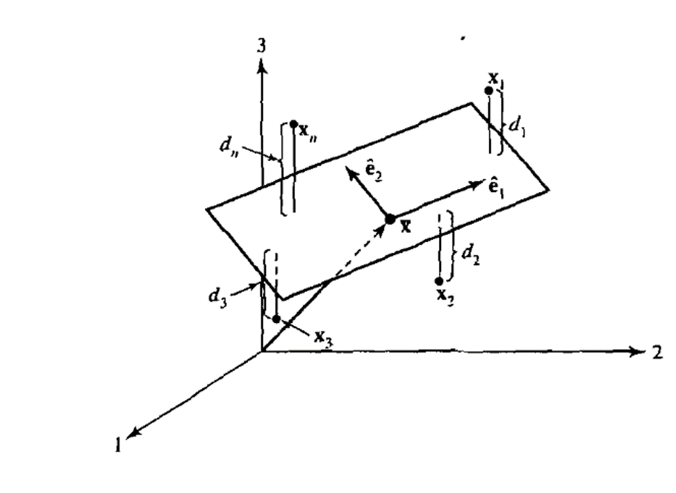
Figure 8.1: The \(r=2\) dimensional plane that approximates the scatter plot by minimising the sum of square deveiations. Reproduced from Johnson, Wichern, and others (2014), supplement 8A, page 469$
Algebraically the gemetric argument starts with some definitions:
Definition 8.3 (r-dimensional hyperplane) All points \(\underset{(p \times 1)}{x}\) lying in an r-dimensional hyperplane through the origin satisfy: \[x=b_{1}\underset{(p \times 1)}{u_{1}}+b_{2}\underset{(p \times 2)}{u_{2}}+ ...+b_{r}\underset{(p \times 1)}{u_{r}}=\underset{(p \times p)}{U}\underset{(p \times 1)}{b}\]
for some b.
All points \(\underset{(p \times 1)}{x}\) lying in an r-dimensional hyperplane through a point \(\underset{(p \times 1)}{a}\) satify the equation:
\[x=a+Ub\]
\(\square\)Definition 8.4 (geometric definition of objective function in PCA) Lets denote the approximtion to the jth observation \[\widehat{x_{j}}=a+Ub_{j}\]
Our objective in PCA is to find the matrix/hyperplane \(U\) which minimises the squared distance \(d_{j}\) between observations and their approximation. We seek to minimise:
\[\sum_{j=1}^{n}d_{j}^2=\sum_{j=1}(x_{j}-a-Ub_{j})^´(x_{j}-a-Ub_{j})\]
where \(d_{j}:=x_{j}-a-Ub_{j}\) and \(\sum_{j=1}^{n} b_{j}:=0\).
\(\square\)Applying the minimisation result from Proposition 8.1 for the error sum of squares, we can now make the following geometrical argument (see Johnson, Wichern, and others (2014), page 468). It states that the best approximating r-dimensional plane is spanned by the first r-eigenvectors of S. Each p-dimensional data point is approximated by its projections onto these eigenvectors.
where the inequality follows from the previous minimisation lemma. Minimisation occurs where \(a=\overline{x}\) and \(Ub_{j}=\widehat{E_{r}}\widehat{E_{r}}^´(x_{j}-\overline{x}))\)
\(\square\)In PCA the value of the projection of an observation onto the i-th eigenvector is given a special name, “the ith principal component” (see Johnson, Wichern, and others (2014), page 432):
Definition 8.5 (The i-th principal component) Let \(\underset{(p \times p)}{\Sigma}\) be the covariance matrix associated with random vector \(Z=[Z_{1},..,Z_{p}]\). Let \(\Sigma\) have the eigenvalue, eigenvector pairs \((\lambda_{1},\underset{(p \times 1)}{e_{1}}),....,(\lambda_{p},\underset{(p \times 1)}{e_{p}})\) where the eigenvectors are ordered from largest to smallest. Then the ith principal component is given by:
\[Y_{i}=e_{i}^´Z\]
Furthermore this means that:
\[\begin{align} Var(Y_{i})&= e_{i}^´\Sigma e_{i} = \lambda_{i} \\ Cov(Y_{i},Y_{k})&=e_{i}^´\Sigma e_{k}=0 \end{align}\] \(\square\)The contribution of the ith principal component to the total sample variance is \(\lambda_{i}\).
References
Johnson, Richard Arnold, Dean W Wichern, and others. 2014. Applied Multivariate Statistical Analysis. Vol. 4. Prentice-Hall New Jersey.