Chapter 8 Examples of ENA models

In this chapter, we will dive deeper into the Shakespeare dataset and develop three ENA models. Also, we are going to suggest some code elimination techniques and ways of interpreting an ENA model. The Shakespeare dataset is available here ??.

8.1 Short summary of the Shakespeare plays

The key of ENA model interpretation is a deep knowledge of the data and its coding. Formal introduction into the data formatting and coding process is described in Chapter ??. In this subchapter, we are going to focus on the content of the two Shakespeare plays to help interpret the ENA models as described in the following subchapters.

8.1.1 Hamlet

After Hamlet’s father passes away, his mom marries his father’s brother Claudius. One day, a ghost appears in the castle, claims to be Hamlet’s father and tells Hamlet that he was murdered by Claudius. In response to that Hamlet plans to revenge his father and kill Claudius. The first part of his plan is to pretend to be insane. He hires some actors to reenact the murder of his father. During the play Claudius gets very mad, which confirms his guilt to Hamlet. Hamlet attempts to kill Claudius, but instead kills his girlfriend’s father Polonius, which results in her committing suicide. Claudius and Polonius’ son, Laertes, plot to poison Hamlet with wine. Hamlet’s mom drinks the poisoned wine by accident and dies. During Laertes’ and Hamlet’s fight, Hamlet gets injured with a poisoned sword and kills Laertes. Afterwards, Hamlet kills Claudius and dies himself (see also Figure 8.1).

One page summary of the Hamlet play ([source](https://goodticklebrain.com/home/2020/9/29/a-stick-figure-hamlet-one-page-summary))

Figure 8.1: One page summary of the Hamlet play (source)

8.1.2 Romeo & Juliet

Two families are in conflict, the Montagues and the Capulets. Romeo Montauge sneaks into a ball to see a girl that he is in love with, Rosaline Capulet. He sees there Julia and falls in love with her. They meet at her balcony and decide to get married in secret, as their families would never accept their relationship. Romeo kills Juliet’s cousin in revenge of him killing his friend. As a consequence he is banished from the city. Juliet is told to marry Paris. She does not want to do it, because she is already married to Romeo. Juliet and the priest that married her and Romeo come up with a plan. She will pretend to be dead, Romeo will come back and they will run away together. However, Romeo did not receive the message that Juliet is just faking her death. He really thinks that she passed away. Next to her tomb, he kills Paris, and then drinks poison. When Juliet wakes up and sees Romeo dead, she kills herself. At the end of the play, two families decide to stop fighting. (see also Figure 8.2).

One page summary of the Romeo & Juliet play ([source](https://goodticklebrain.com/home/2017/7/18/romeo-and-juliet-one-page-summary))

Figure 8.2: One page summary of the Romeo & Juliet play (source)

8.2 Model 1: Differences in discourse between two plays

In the first model we are going to examine main differences between the Romeo & Juliet and Hamlet plays (for more information about the Shakespeare dataset go to ??). To do that we will explore some code elimination techniques. Notice that the list of techniques listed here is not exhaustive and may not match your particular dataset or research question.

Setting up the model

To start with, we are going to develop a model based on the Shakespeare dataset with the following specifications (see Figure 8.3):

Units: Play > Act > Scene > Speaker
Conversations: Play > Act > Scene
Codes: All
Comparison groups: Plays
Stanza window: 4

We removed the plotting point to focus only on the connections between the codes (refer to Subchapter 2.1 for Unit selection). To generate a substraction network for two plays, click on the means of the plays (go to Subchapter 2.4 for more information on Means options).

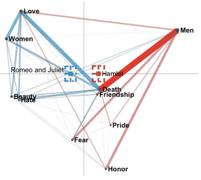
Figure 8.3: Base model

If your model does not look exactly as the one above, check Chapter 5.1 on Dimension options - you might need to flip the axes of your model. For other aesthetic options, such as increasing the edge or text size, see Chapter 5.

By looking at the subtraction model above, we can already get some idea about the differences between two plays. The red edges represent stronger connections for the Hamlet play, while the blue ones for the Romeo & Juliet. The goal of the ENA is to not only to visualize the data, but also to close the interpretative loop, deeply understand the data behind the model and the story told. In the next couple of steps, we will try to “clean” the base model and try to use the least amount of codes to convey the meaning behind the data. Remember that you should be able to justify any decision that you make regarding your model.

1. Codes close to each other

One criteria that can help you eliminate codes is to exclude codes that are close to each other. Examples of that in our model are Beauty and Hate (refer to Figure 8.3). If the codes are close to each other, it means that both codes come up together a lot within one stanza, and keeping both of them might not add much value to the model. To choose a code to eliminate, you should examine, which code bares more meaning to your research question. In the case of our model, we eliminate Beauty, as Hate seems to be more meaningful, since the opposite of Hate, i.e. Love, has some strong connections to other codes (see Figure 8.4 for a model without Beauty).

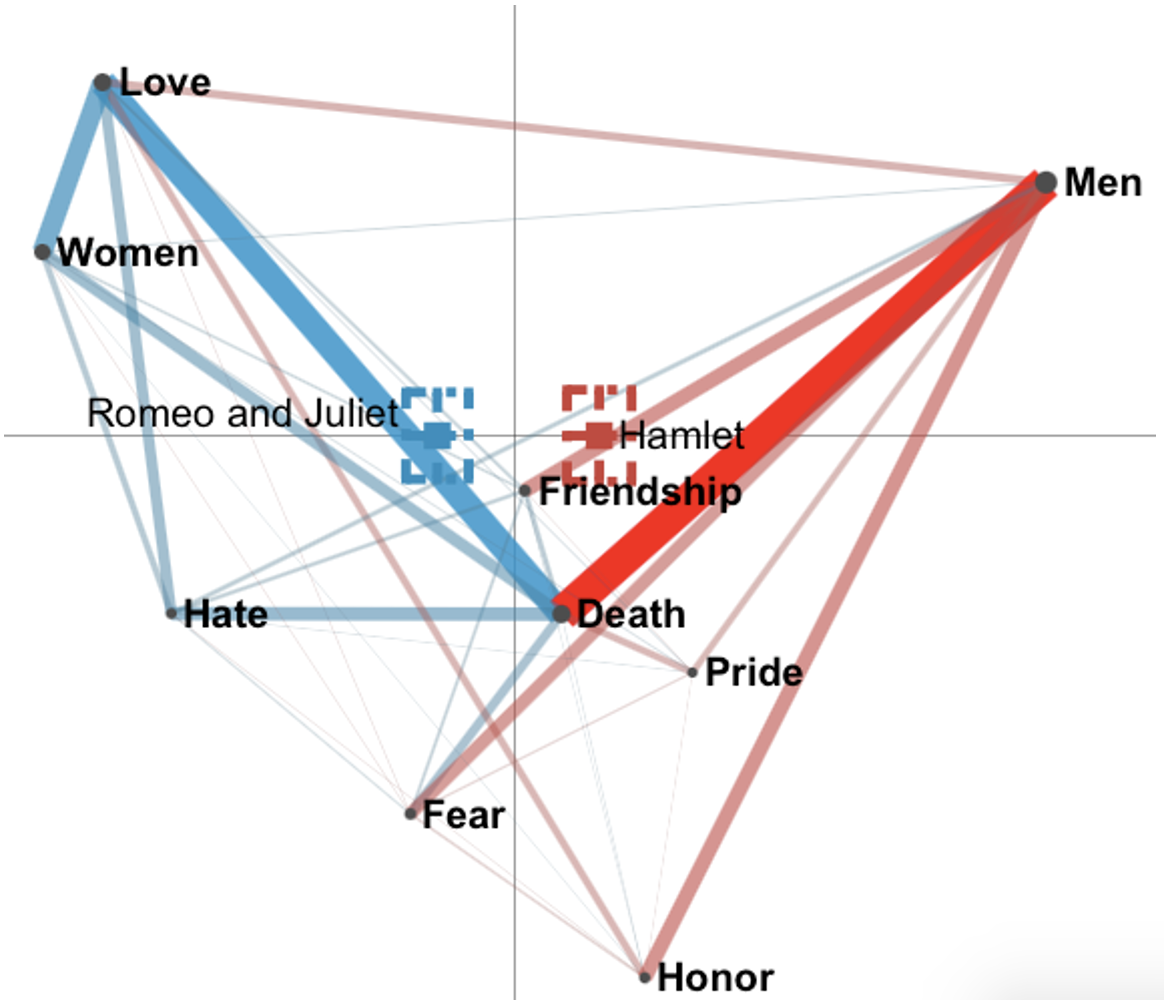
Figure 8.4: Shakespeare model without Beauty

2. Weak connections with other codes

Another way of determining an exclusion of a code, would be to look at the strength of its connections with other codes. Some codes are weakly connected, which indicates that the difference between two comparison groups are small. In our model Pride has weakest connections to other codes. If you compare Figure 8.4 with the Pride code and 8.5 without Pride, you can see that the model did not change much after the exclusion.

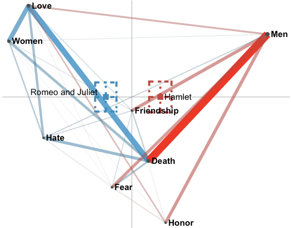
Figure 8.5: Shakespeare model without Beauty and Pride

3. Code centrality

The centrality of a code can have two meanings:

it indicates that the central code is shows a crucial difference between the comparison groups through its connections to the other codes,
or it does not add much value to the model by not exposing more significant differences between the codes.

In our model, we have two codes that are central Friendship and Death. Figure 8.6 shows a model without Friendship and another model without Death. By eliminating either of these codes, we get a different story from our data. It seems that Death is a distinguishing code between two comparison groups, while Friendship divides the codes into two groups with stronger connections for each play.

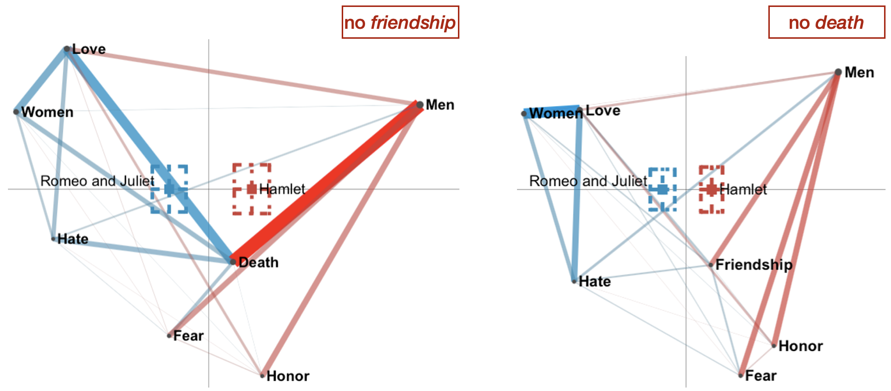
Figure 8.6: Shakespeare models without Beauty, Pride, and Death or Friendship

4. Model interpretation

You can also make some executive decisions based on your research question and remove codes that do not add value to your data story. However, you must be able to justify the decisions that you make.

For example, we remove Honor from our models from the precious subchapter, as this code does not highlight any significant differences between the plays - its stronger connections with other codes are only for the Hamlet play (see Figure 8.7).

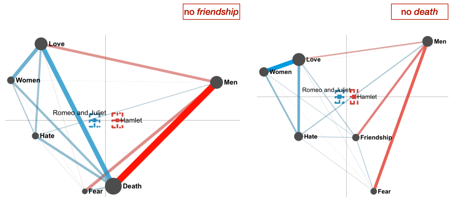
Figure 8.7: Shakespeare models without Beauty, Pride, Honor, and Death or Friendship

5. Statistics

Finally, you can look at the statistics of each model and base your code elimination decisions on that. Table 11.1 shows differences in variance explained by the models and goodness of fit statistics for each model as developed in precious subchapters (see Figure 8.7). Based on the statistical analysis, Model with Friendship explains more variance on the Y-axis and better fits the model, as it has higher co-registration correlation for both dimensions (Spearman and Pearson goodness-of-fit tests), while Model with Death explains more variance on the X-axis. According to these results, some might decide for the Model with Friendship.

Table 11.1. Statistics for two Shakespeare models without Beauty, Pride, Honor, and Death or Friendship

\[ \begin{matrix} \begin{array}{c|c|c|cc|cc} \text{} & \text{MR1} & \text{SVD2} & \text{Pearson} & & \text{Spearman} \\ \text{} & \text{} & \text{} & \text{X-axis} & \text{Y-axis} & \text{X-axis} & \text{Y-axis} \\\hline \textbf{Model with Friendship} & \text{10.8%} & \text{29.3%} & \text{0.94} & \text{0.82} & \text{0.95} & \text{0.82} \\\hline \textbf{Model with Death} & \text{14.1%} & \text{21.6%} & \text{0.90} & \text{0.77} & \text{0.89} & \text{0.77} \\\hline \end{array} \end{matrix} \]

If you are interested in mathematical methods of removing codes, check the article on the Parsimonious Removal with Interpretive Alignment of the ENA codes by Wang, Swiecki, Ruis, & Shaffer (2021).

Closing the interpretative loop

What are the differences between the Hamlet and Romeo & Juliet plays? We developed two models to answer this questions (see Figure 8.7).

The strongest connections in the Model with Friendship for the Romeo & Juliet play are Women-Love , Hate-Love, and Women-Hate. In comparison, the strongest connections in the Model with Death for the Hamlet play are Men-Fear , Men-Friendship, and Love-Men. Romeo & Juliet is more centered around the love story (Women-Love), but the topic of love exists in the context of the family feud (Hate-Love, Women-Hate). One of the biggest themes in Hamlet are friendships between men, for example Hamlet’s friendship with Horatio, or the fake friendship between Hamlet and his two childhood friends, who were spying on him (Men-Friendship). Fear is strongly connected to men in Hamlet, such as Hamlet fearing the king (Men-Fear). However, in Hamlet men are also connected with love, as in the case of Hamlet’s love to his father or Leartes’s love to his father (Love-Men).

Model with Death has similar connections for Romeo & Juliet (Women-Love, Hate-Love) and Hamlet (Love-Men, Men-Fear), but it is the connections to Death that show the biggest difference between the plays. In Romeo & Juliet Love-Death connection has two reasons. On one hand, it is a love story with a suicide at the end. On the other hand when the characters talk about their love, they become a bit melodramatic about its intensity. In Hamlet Men-Death is the strongest connection. Death is present through many murders, attempted murders, or plotting about committing a murder. Moreover, the character of a ghost adds to the Death theme.

These two models tell two different stories about the Romeo & Juliet and Hamlet plays. While Model with Friendship divides plays’ themes, Model with Death strongly contrasts them.

8.3 Model 2: Trajectory model by acts

In this subchapter, we are going to develop networks for every Hamlet act and compare the 2nd and the 4th acts (for more information about the Shakespeare dataset go to ??). Also, we go into depth of interpreting ENA trajectories.

Setting up the model

To start with, we are going to develop a model based on the Shakespeare dataset with the following specifications (see Figure 8.3):

Units: Play > Act > Scene > Speaker
Conversations: Play > Act > Scene
Codes: All
Comparison groups: Plays
Stanza window: 4

We removed the plotting point to focus only on the connections between the codes (refer to Subchapter 2.1 for Unit selection), and excluded Romeo & Juliet play (refer to Subchapter 2.6 for Excluding units). Afterwards, we selected means for each individual act in Hamlet and removed the confidence interval for the Hamlet play mean (refer to Subchapter 2.4 for Mean options), and change means’ colors for better readability (refer to Subchapter 2.8 for Unit color changing). After generating the plot for the whole Hamlet play by clicking on the Hamlet play mean, we ended up with the model depicted in Figure 8.8).

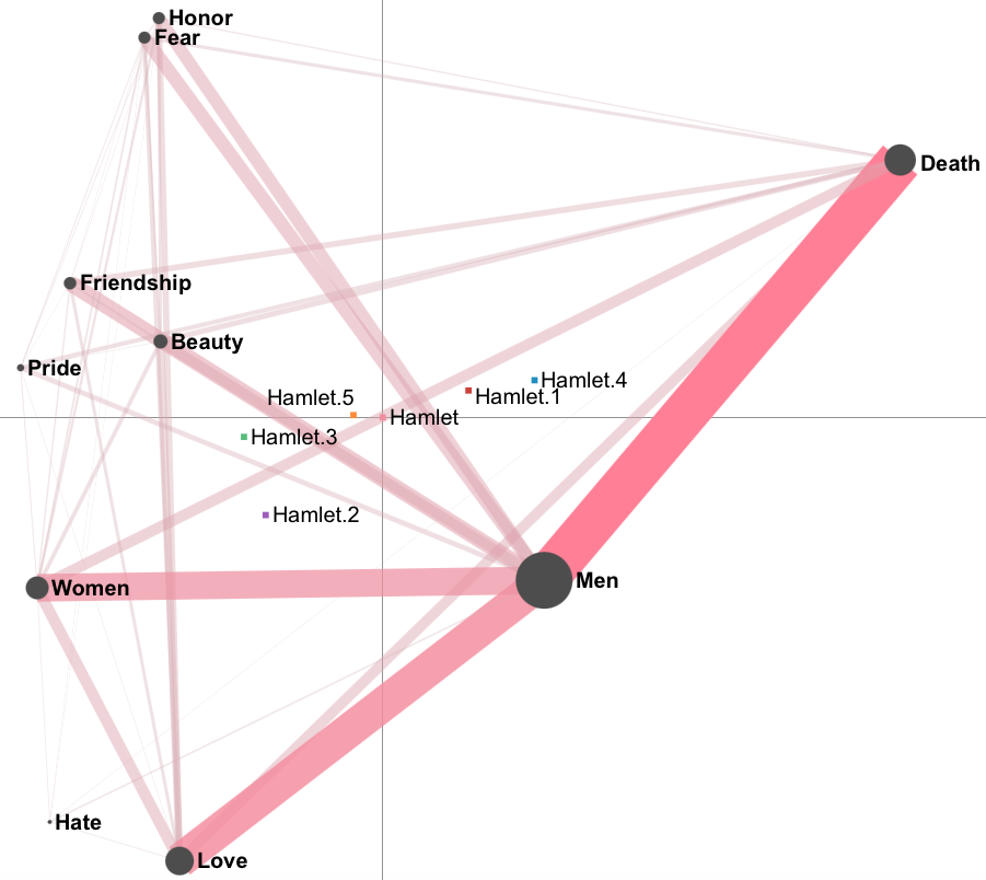
Figure 8.8: Trajectory model for the acts in the Hamlet play

The pink edges represent the connections between the codes for the whole play. The Hamlet mean is in the center of the visualization, while the means for each act are distributed across the graph. The closeness of a mean to particular code connections signifies that they appear often in the particular acts. A visualization of the means for “smaller” units can help visualise a change in the data over time or in different conditions. In the case of Hamlet, it seems like the discourse start in a similar place, where it ends, and during the play explores different themes.

Closing the interpretative loop

Now we are going to compare two acts that are set on the opposite ends of each other - act 2 and act 4. To do that we will click on the means of both acts to get a subtraction network (see Figure 8.9; refer to Subchapter 2.4 for Mean options).

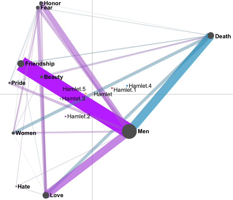
Figure 8.9: Comparison of the 2nd and 4th acts of the Hamlet play

When we examine the model for act 2, we immediately notice a strong Men-Friendship connection. By examining the data, we learn that in this act Hamlet was spied by two of his childhood friends to examine his odd behavior. In contrast, act 4 is dominated by the Men-Death connection, as it is a chapter, where Claudius and Laertes plot and try to kill Hamlet, and Ophelia with her brother grieve the death of their father. Moreover, Ophelia commits suicide in this act (Women-Death).

By comparing different acts, we can see how much each act contributes to the connections for the Hamlet play, and it can help you dive deeper into the data. If you would like to learn more about ENA trajectories, check Trajectories in Epistemic Network Analysis by Brohinsky, Marquqrt, Wang, Ruis & Shaffer (2021).

8.4 Model 3: Comparison between individuals

In this subchapter, we are going to develop individual networks for the characters of Ophelia and Juliet and compare them in the context of both plays (for more information about the Shakespeare dataset go to ??). Also, we will explore models rotated by the mean and not, and dive into its implications.

Setting up the model

To start with, we are going to develop a model based on the Shakespeare dataset with the following specifications:

Units: Speaker > Play > Act > Scene
Conversations: Play > Act > Scene
Codes: All
Comparison groups: Ophelia, Juliet
Stanza window: 4

We removed the plotting point to focus only on the connections between the codes (refer to Subchapter 2.1 for Unit selection). We developed two subtraction networks by clicking on the means for Juliet and Ophelia, and setting the means rotation either to by Ophelia and Juliet or turning it off (see Figure 8.10; refer to Subchapter ?? for Mean rotation).

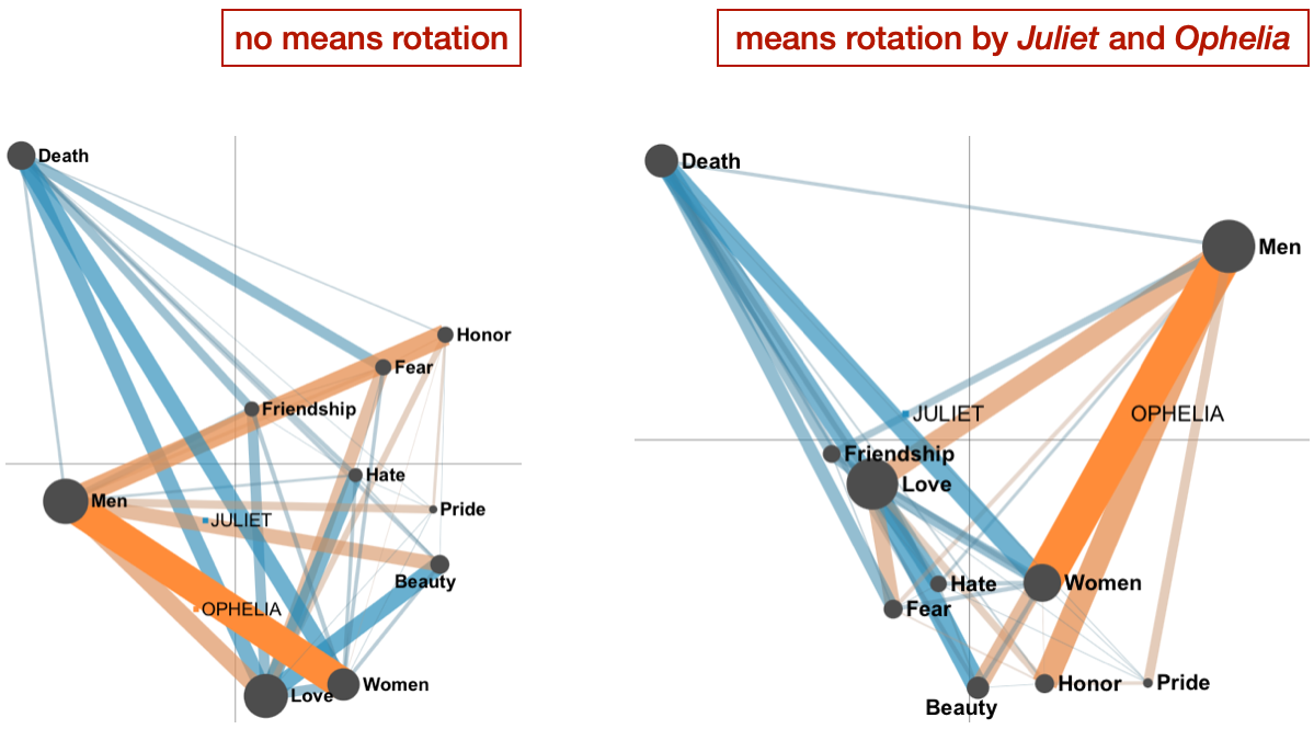
Figure 8.10: Comparison models of Ophelia and Juliet with and without the means rotation

Closing the interpretative loop

To compare Juliet and Ophelia, let’s start with some background. Both of them are main love interests in their plays and both commit suicide. When we take a look at the comparison networks, we notice that Ophelia connects Love with Men and Fear, while Juliet with Death and Beauty (see Figure 8.10). It indicates the darker love story inn Hamlet that included rejection Ophelia by Hamlet, and more of a typical melodramatic love story in Romeo & Juliet. When we look at the mean of Juliet’s network, we can see that it is pulled between Death and Love as two polar opposites, while Ophelia is pulled between Men and Honor, Beauty, and Pride. Though Ophelia also commits suicide, the topic of Death is not dominant in her discourse in connection to other codes. Similarly, Juliet’s discourse does not center Men in connection to other codes, with exception of Death and Hate.

What does the means rotation do or help with? What to watch out for? (in the context of model interpretation)