Chapter 3 Working with Data
What is data? Data is a term we all use probably many times a day but it is worth stopping to think about what it actually means. The first use of data occurred in 1646 and etymologically the term data comes from the word given. Data is traditionally plural of the term datum, although both terms are oftentimes used interchangeably (and possibly incorrectly).
3.1 Motivating Data Collection and Management
Data describe. They document the who, what, where, when, and why. We are increasingly understanding the motivations for good data collection and good data management. First off, very complex problems require data synthesis. For instance it is hard to solve long-term and or large-scale challenges (think: climate change) without combining different datasets. In the same way, data are valuable beyond the current project often in ways we can’t predict. Most results from scientific studies are not transparent enough to be repeated, which would be inefficient to begin with (Michener and Jones 2012), but which also underscore the need for good data management. Another important consideration is to preserve and publish our dataas a means to make data available to others in the future (Rüegg et al. 2014). All of the attention that good data collection and data management require point to the fact that data management should be funded. That’s a topic for another time; however, the efforts and focus that go into data collection and data management should not be dismissed.
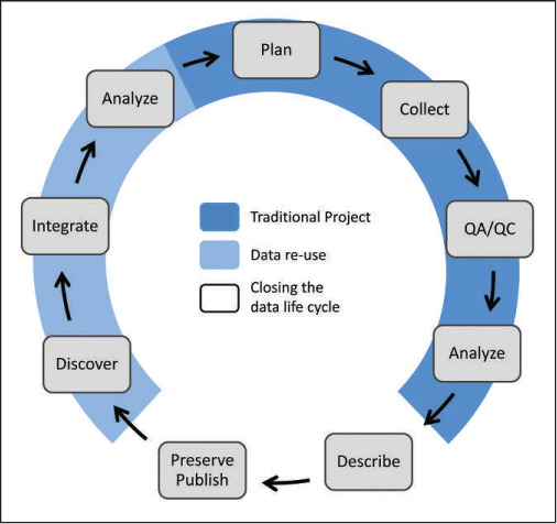
Figure 3.1: The data lice cycle (Rüegg et al. 2014)
3.1.1 Historic data collection
Data has often been recorded in unique and idiosyncratic ways. This includes both structural and technologically different ways along with their limitations. Structurally, the dependence was on what was being recorded. For example, field notes or some version of field notes were often the only type of data that was recorded for many centuries. Although the idea of field notes may seem ancient it is still very much encouraged to record field notes. The technological recording of data has advanced greatly not only in the past few years but in the past few 100 years. Tally sticks for messaging or recording debts represent some of the earliest data recording structures that we have. Clay tablets and papyrus are other forms of ancient data recording. The printing press was a major advancement not only for books and the printed word, but also for how data were shared or made available (aren’t books just character data?). Fast forward to more recent times and we have physical recordings of data like punch cards. From there we have magnetic storage, which came in the form of floppy disks and disk drives. And more recently we have flash storage and cloud storage.
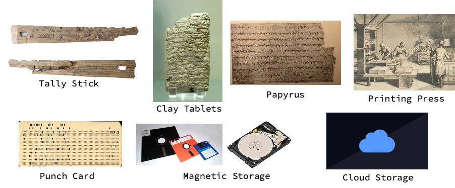
Figure 3.2: Evolution of data recording (Source: Wikipedia).
3.1.2 Data recording today
Today most data is recorded (or ends up) electronically in a spreadsheet, which is often a Microsoft Excel file. Spreadsheets are visually accessible and a common way to share data that take the form of rows and columns. It’s worth noting that a Microsoft Excel file is a proprietary file format, and while it may have very good applicability in certain instances using a non-proprietary file format is advised. Examples of non-proprietary file formats include text files (.txt) and comma separated values files (.csv). Text files underlie most of the non-proprietary and robust file types that are recommended and CSVs are just a form of text files that use commas to separate columns. Not only are these non proprietary file types more accessible to a greater number of software, they are also generally more resistant to corruption because they lack a lot of the additional formatting that comes with Microsoft Excel files and other proprietary file types.
3.1.3 A word about Excel
Although Microsoft Excel can be a very useful software there are some concerns about using Excel in quantitative settings. First off Excel is not a statistical software. Yes, it can do certain statistical functions but ultimately it’s not a software that most quantitative analysis will will use. Excel has the ability to store multiple tables (or multiple worksheets) in one file and while this may be useful in certain instances this type of document structure does not work well with R. Similarly you may have used highlighting or other annotation tools within Excel. While this may be effective it does not translate into R, which requires simply a flat file with alphanumeric information in it. You may also have done calculations within a cell in an Excel spreadsheet. An example of this would be where you may have a number in a certain cell but when you click on that number you see that the formula bar indicates that something (often a formula) is going into creating or referencing that number. That is a problem for R because R simply needs one value per cell and doesn’t work with Microsoft Excel formulas. Another concern with Excel is that the metadata are often implicit within one file. Of course they need not be and metadata can exist in other files but oftentimes the highlighting and annotation is a form of metadata or information transfer that takes the place of actual metadata. See the article by (Mélard 2014) for a discussion of this topic.
3.2 Data Recording suggestions
There are a number of simple and common approaches to improving how we record data. What follows are some tips, which need not be adopted every time and may not be an exclusive list but are a good reminder of the simple things we can do to improve our data management. Also, please see (Borer et al. 2009) for more details on this topic.
Use a useful file name. Consider time, place, or study term that may help describe what is in the data file. You don’t need the file name to be extremely long, but short file names, like mydata.csv, may also be vague and unhelpful. It is recommended not to use spaces or dots in a file name because the dot indicates the separator of the file type from the file name. Camel caps are a suggested alternative (e.g., “LakeFishStudy2020.csv”), such that spaces and underscores don’t need to be used but the file name still has readability.
Record or input your data close to the time of collection. This is exactly as it sounds because you (or your colleague, your technician, or someone else) will likely forget information about how the data were collected or other relevant pieces of data the longer you are away from your data.
Standardize how you record your data. For example, if you are including species names in your data pick a convention like
Gspecies, orgenus_species, orGs. Pick one format, document it in the metadata, and stick with it so that there’s no confusion how similar types of data are being recorded within the same data file.Keep raw data raw. Record data in its most basic form. Raw data may include copies of a field notebook, photographs of data in a field notebook, or just a raw file such as an Excel file of the first input of the data—warts and all. However, after that you will use a copy of the raw data to clean it up, manipulate it, and otherwise get it into R for analysis. The one caveat to keeping raw data is that you also want the characters to be raw; in other words, don’t include symbols or accents or any other typography that is not found on your keyboard.
When in doubt make multiple columns. In other words split your data and don’t lump it together. A common example of this would be if you have a
datecolumn in your data; consider splitting it into columns separate forday,month, andyear. Splitting this way allows you to use thedateif needed, but also subset your data by themonthin which it was collected, which may be a relevant factor. You can always reconvene data that have been split but if things are lumped together and they’re not split there may come a time when you forget how they can be split.Consider a universal formatting for data inputs. You may want to have some type of format or style for your column headings. An example of that might be using all uppercase letters for your column headings; e.g.,
SAMPLE,TREATMENT, etc.. Again don’t use spaces or dots. This is not particularly important other than having a certain formatting that stands out may help you later on when you code because you may be able to more readily identify vectors or other data inputs from the actual variables themselves.Limit one type of information per column. This was indirectly mentioned above regarding splitting (and not lumping) your data. However, what is meant here is literally keep one data type within your column. A data type may be numeric or character data, for example, and it is advised not to mix those. For instance, within a certain column every value in that column should be a number or a character but not a mix of numbers and characters.
Consider a key ID or a unique record indicator. A key idea is often the first column in a data set and it may do nothing more than simply identify each row by giving it a unique identification code. Each row may seem unique to you because it concerns an observation; however, it can still be useful to give that observation an identification number, refered to as a key ID.
Keep an eye on dates. Be careful of dates while using Microsoft Excel. It is advised to use
YYYYMMDDformat and to separate the date into separate elements as described above. Microsoft Excel has the ability to format dates in a wide variety of formats and some of those formats do not translate well to other software like R. This is just something to be aware of as we all struggle with dates at some point.
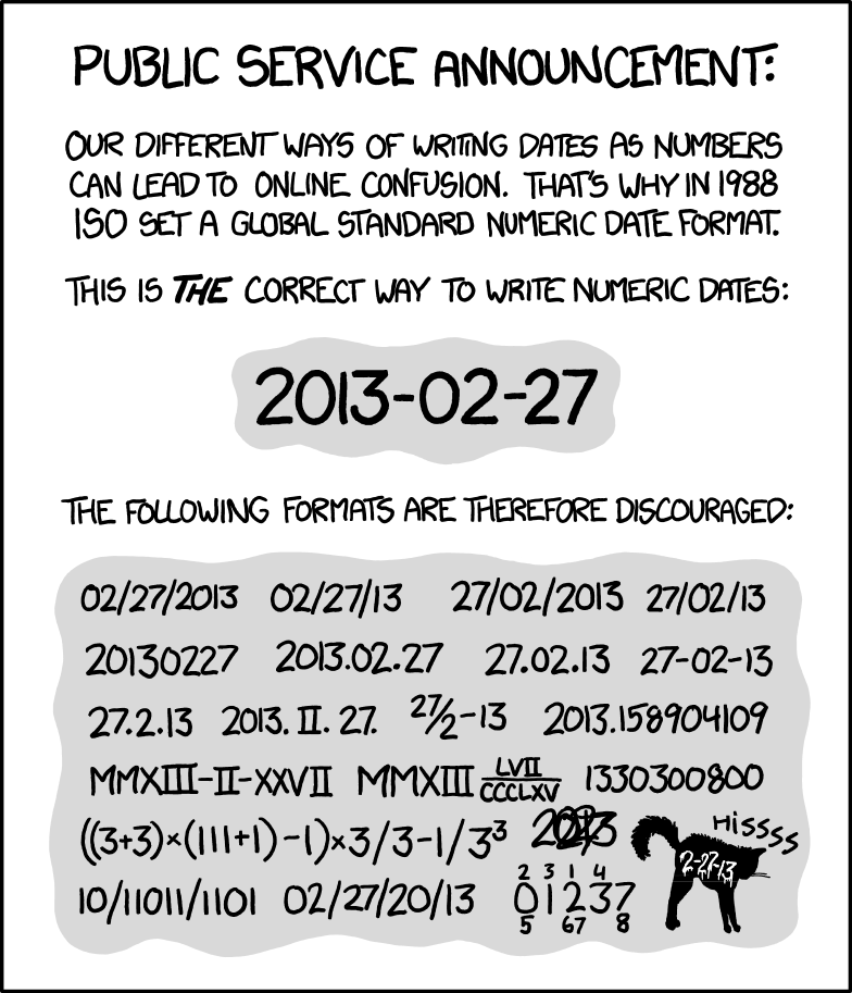
Figure 3.3: Source: XKCD
3.2.1 Tidy data
A lot of the suggestions found in this chapter point to the idea of tidy data. Tidy data is a standardized way of mapping the meaning of a data set to its structure. A data set is messy or tidy depending on how the rows columns and tables are matched up with observations. The three rules of tidy data are presented below, and you are encouraged to check out the full article on this topic for great insights on data organization (Wickham et al. 2014).
The three rules for tidy data include
Each variable forms a column.
Each observation forms a row.
Each type of observational unit forms a table.
(Borer et al. 2009) also presents some good examples (with images) of correcting messy data.
3.3 Data files organization
You may be thinking: there are not only data files, but raw data files and metadata files and other files associated with one single analysis. So how do we organize all those files within one folder? While there is no one correct way to do it there are some general ideas and guidance about how to efficiently organize files associated with one analysis, particularly in R. One such organizational model seen in the image below includes data files, raw data files, and metadata files that are in the same folder as in our script, which may then produce model output or plots or new data. (We may also knit elements of the analysis together in an R Markdown file.) While you need not know all the file types and nuances presented in the image below, the larger point is to keep files together when they are associated with the same project. Keeping them together can literally be as easy as putting them all in the same folder. Opening your R script from that file will set up your working directory to be that same folder (which R calls the working directory), in which the data are also stored. This will alleviate the need to specify file paths and other things that simply add code, create chances for error, and make code less collaborative.
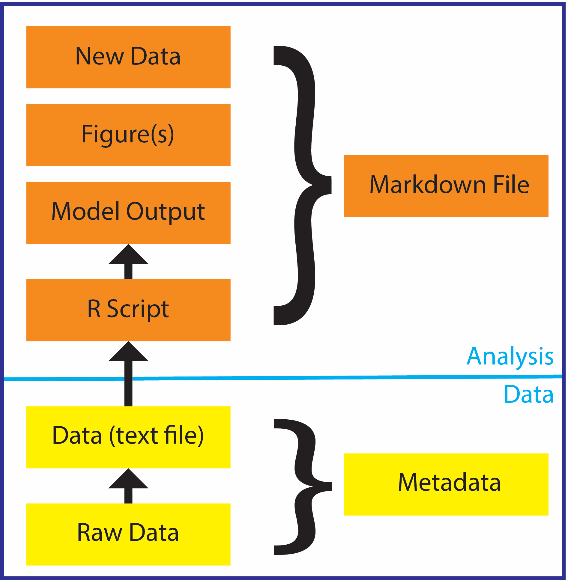
Figure 3.4: Basic file structure.
3.4 Metadata
We have used the word metadata without really defining it; however, metadata can be incredibly important. Metadata is a set of data that describes and gives information about the data. In other words, metadata is like a readme file for your actual data file. Think of metadata as a text file that describes the data types, columns, and intentions of the sampling that created the data that you would like to analyze. Metadata can be incredibly useful because it stores the details that you might (or will) forget. It contains the information that applies to all the data but isn’t replicated in the actual data file. For example you may have all of your sample sites within a given state and as such there may not be a variable in your data for state . However, it could be useful to others who don’t know your data set to know that all of the sampling occurred within one state. On that note, metadata allows other users to understand what is in the data file and, in fact, metadata should be written for the naive user assuming they do not know anything about your study and the data that you’ve collected. Metadata should also be dated regarding changes to the data file, ultimately functioning as a diary or journal for the data such that you can make time specific comments about things that may have been changed. Metadata can take the file type of a simple text file for maximum simplicity, or can be done using XML (Extensible Markup Language), which is a common file type for electronic metadata records.
A good overview of metadata can be found in (Fegraus et al. 2005).
Although you are encouraged to review different metadata to understand what goes in metadata there are some common metadata information that most metadata would have. This information includes:
The person recording and/or imputing the data if there are two different people.
The date of the recording.
The source of the data, if it was not collected by you or is not clear who collected it.
A general time and location such as the date or month or year and the location in which the data were collected, if this information is not included in the data file.
Specific descriptions of all the column names as well as the column data types. This is often refered to as the data dictionary, and can be a stand-alone file. For example you may have a column name called
DgFand it’s wise in the metadata to define this as degrees Fahrenheit. Then, within that degrees Fahrenheit column you would have data types that are numeric or integer based on the resolution of recording.Include units. Units may be included subtly within the column names (a good idea); however, it’s really important to include the unit types within the metadata at least as a backup. You will likely find yourself abbreviating things in the data, which is fine, but use the metadata to define and explain the abbreviations.
A description of how missing elements are notated. Are missing elements of data notated with an
NA, or a99, or a dash, or a blank cell? All of these are ways that people have indicated missing elements. Generally speaking it is best to leave a cell blank if there’s missing information, but regardless of what you choose just make sure you include it in the metadata.
3.5 Data Archiving Suggestions
When it comes to recording data there’s a few final and common sense suggestions.
Obviously make sure your data is machine readable–this does not even need to be said in the 21st century. There are a lot of advantages to having physical copies of data but ultimately the data needs to be in digital form such that it can be read by one or more statistical software.
Keep your data secure, which means backup your data. A rule commonly associated with backing up your data is the 3-2-1 Rule, which means having at least three total copies of your data, two of which are local but on different devices, and at least one copy off-site. Other rules may also work, but the ideas are typically the same.
Adhere to your data management plan (DMP) if you have one. Producing outcomes that adhere to your data management plan will be much easier if you make little steps along the way rather than at the project end trying to refit everything you’ve done data wise to the data management plan. Also, if you put strategy and thought into your DMP, it should make your data management easier!
Although this has been stated earlier: use non-proprietary and open formats to save your data. While Microsoft Excel has its strengths and can be useful in some applications it’s best to stick to text files and other file types that are less corruptible and are unlikely to ever undergo major changes.
3.6 Further Reading
Scientific article on data and data management were uncommon just a few years ago. Several good papers have been cited in this chapter, but others are worth mentioning and more are being published all the time. Borghi et al. (2018) present thoughts on data management for researchers, including practical guidance. For some best practices about create a data management plan, see some rule presented by Michener (2015). White et al. (2013) overview practices for sharing data, much of which boils down to good data management. And finally, for some tips on managing data in spreadsheets (including lots of visuals), check out Broman and Woo (2018).