Chapter 8 GLMs: Generalized Linear Models
8.1 Overview
In The Linear Model chapter we discussed different common probability distributions. You are encouraged to reference that section, because ultimately these different probability distributions are at the root of what makes a linear model a generalized linear model (GLM). In other words a generalized linear model is just a linear model, but with a modified error distribution that better captures the data generating process that has helped in the creation of your data. For instance, if your responses are successes and failures, which are typically coded as 1s and 0s, it is pretty clear that 1s and 0s are not normally distributed data nor would they have a normal error distribution on their residuals. In cases like these we need to modify our underlying linear modeling distribution to best match what distribution has helped shape our data.
A GLM will look similar to a linear model, and in fact even R the code will be similar. Instead of the function lm() will use the function glm() followed by the first argument which is the formula (e.g, y ~ x). Although there are a number of subsequent arguments you may make, the arguement that will make your linear model a GLM is specifying the family, which you will set to poison or binomial or whatever error distribution you are applying to this model. It’s also worth noting that each family that you can specify has an underlying default link function. The link function is what transforms the data in the GLM. The identity link (or canonical link) is the default link function and also the link function that you will likely want to use the vast majority of times; however, it’s worth noting that you are able to change the link function to something else should you choose to.
[Table of families and link functions?]
Let’s evaluate a few common GLMs.
8.2 Poisson linear regression
Recall the Poisson distribution is a distribution of values that are zero or greater and integers only. The classic example of Poisson data are count observations–counts cannot be negative and typically are whole numbers. The Poisson distribution has one parameter, $(lambda), which is both the mean and the variance. A Poisson regression uses Log link (and therefore the coefficients need to be exponentiated to return them to the natural scale).
# Simple Poisson GLM
glm(y ~ x, family = poisson)
8.2.1 Poisson linear Regression Example
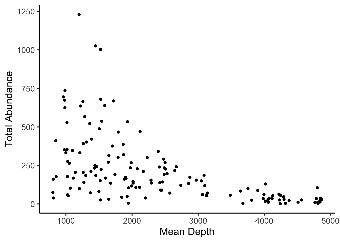
Using the fishing data in the COUNT library, let’s model the relationship between total abundance (totabund) and mean depth (meandepth). Total abundance are counts, and we might hypothesize that abunndances of fishes decreases with increasing depth.
library(COUNT)
data(fishing)
Let’s look at the relationship first, as usual.
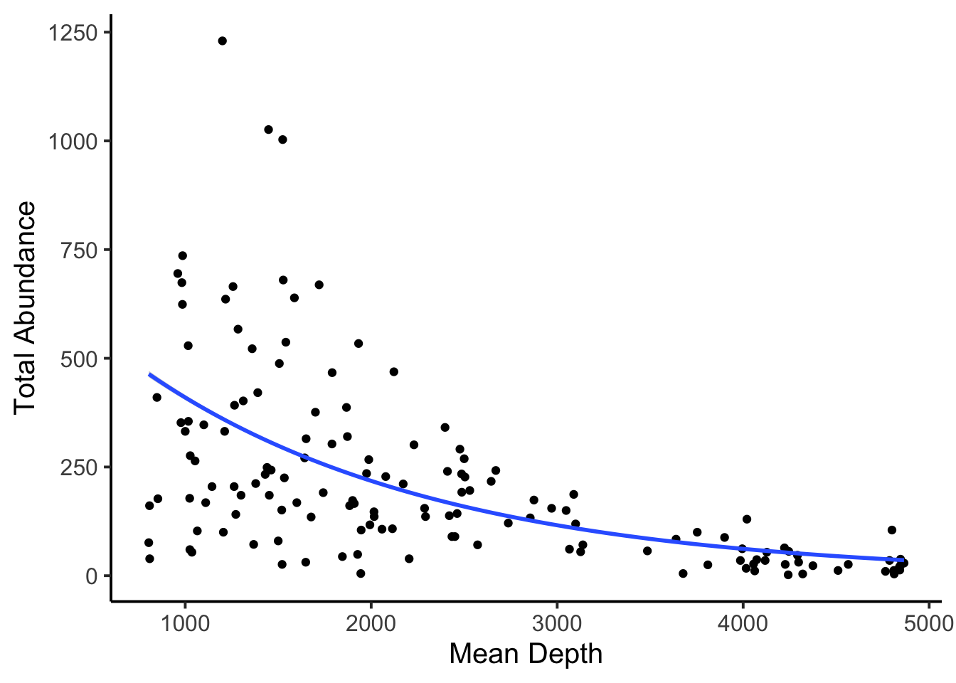
And now let’s plot the model.
pois.glm <- glm(totabund ~ meandepth, data = fishing, family = poisson)
summary(pois.glm)
##
## Call:
## glm(formula = totabund ~ meandepth, family = poisson, data = fishing)
##
## Deviance Residuals:
## Min 1Q Median 3Q Max
## -25.567 -6.824 -2.965 3.771 35.730
##
## Coefficients:
## Estimate Std. Error z value Pr(>|z|)
## (Intercept) 6.647e+00 1.269e-02 523.96 <2e-16 ***
## meandepth -6.309e-04 6.659e-06 -94.74 <2e-16 ***
## ---
## Signif. codes: 0 '***' 0.001 '**' 0.01 '*' 0.05 '.' 0.1 ' ' 1
##
## (Dispersion parameter for poisson family taken to be 1)
##
## Null deviance: 28050 on 146 degrees of freedom
## Residual deviance: 15778 on 145 degrees of freedom
## AIC: 16754
##
## Number of Fisher Scoring iterations: 5The model output looks a lot like our lm() model output—there minimal mention of the poisson part of the regression. The estimated coefficients don’t like numbers we used in the model, but we have to remember that these are estimates on the log scale, so if we back-transform them, we should recover more meaningful numbers.
# Back-transform the intercept
exp(coef(pois.glm)[1])
## (Intercept)
## 770.1425# Back-transform the slope
exp(coef(pois.glm)[2])## meandepth
## 0.9993693The slope may be a little harder to interpret, but the intercept of 770 makes a lot of sense given the plot. Finally, we may want to plot the model.
8.3 Binomial linear regression
Binomial regression is for binomial data—data that have some number of successes or failures from some number of trials. Let’s focus on the most common application of the binomial regression which is that when the number of trials is 1, which is often called logistic regression. The application of this model is when we have 1s and 0s as our outcomes, which often represent successes or failures, presence or absence, or any other binary outcome. The coefficients of a logistic regression model are reported in log-odds (the logarithm of the odds), which can be converted back to probability scale with the plogis() function. It is also worth noting that the estimate of \(p(50)\), or the probability of 50% for \(y\), is calculated simply by taking the fraction of the negative intercept over the slope value.
# Simple binomial GLM
glm(y ~ x, family = binomial)
8.3.1 Binomial Linear Regression Example
Using the YERockfish data in the FSAdata library, let’s model the relationship between fish maturity (maturity) and length (length). Maturity is a binary response (immature or mature), and we might hypothesize that the probability of being mature increases with length.
library(FSAdata)
data("YERockfish")
Before we do anything, there are a few NAs in the data we need to remove, and we also need to convert the maturity data to 1s and 0s.
# Remove NAs
YERockfish2 <- na.omit(YERockfish)

# Convert maturity data into 1s and 0s
YERockfish2$maturity2 <- ifelse(YERockfish2$maturity == "Immature", 0, 1)
Let’s look at the relationship first, as usual. Due to many overlapping data point, the data werre jittered and transparency was increased.
ggplot(YERockfish2, aes(y = maturity2, x = length)) +
  geom_jitter(width = 0.05, height = 0.05, alpha = 0.5) +
  theme_classic(base_size = 15)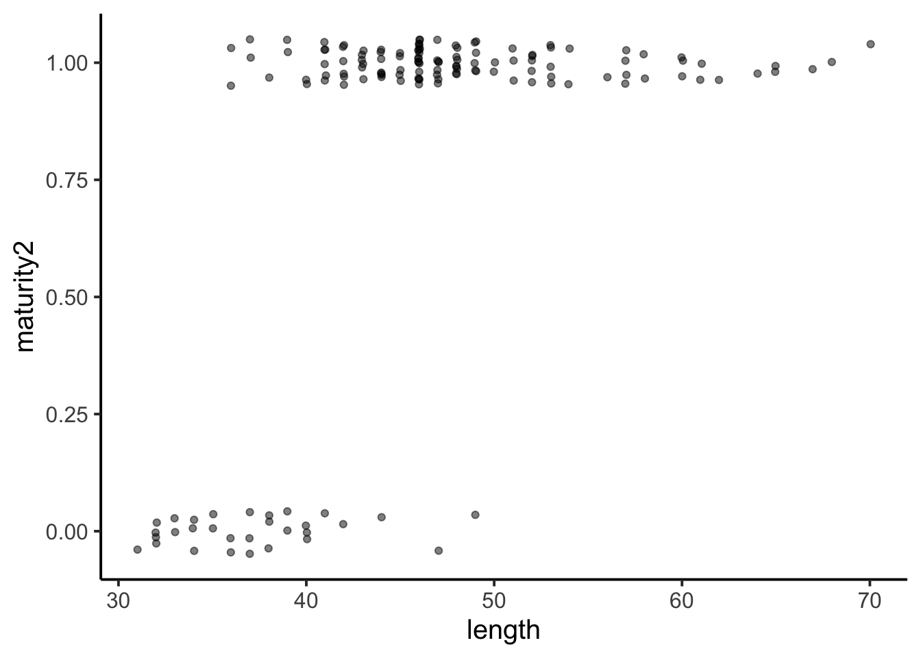
And now let’s plot the model.
binom.glm <- glm(maturity2 ~ length, data = YERockfish2, family = binomial)
summary(binom.glm)
##
## Call:
## glm(formula = maturity2 ~ length, family = binomial, data = YERockfish2)
##
## Deviance Residuals:
## Min 1Q Median 3Q Max
## -2.99343 0.00994 0.18751 0.35685 1.71455
##
## Coefficients:
## Estimate Std. Error z value Pr(>|z|)
## (Intercept) -16.93066 3.23684 -5.231 1.69e-07 ***
## length 0.43673 0.07993 5.464 4.65e-08 ***
## ---
## Signif. codes: 0 '***' 0.001 '**' 0.01 '*' 0.05 '.' 0.1 ' ' 1
##
## (Dispersion parameter for binomial family taken to be 1)
##
## Null deviance: 148.767 on 146 degrees of freedom
## Residual deviance: 73.987 on 145 degrees of freedom
## AIC: 77.987
##
## Number of Fisher Scoring iterations: 7The model output looks a lot like our lm() model output—there minimal mention of the binomial part of the regression. The estimated coefficients don’t like numbers we used in the model, but we have to remember that these are estimates on the log scale, so if we back-transform them, we should recover more meaningful numbers.
# Back-transform the intercept
plogis(coef(binom.glm)[1])
## (Intercept)
## 4.437195e-08# Back-transform the slope
plogis(coef(binom.glm)[2])## length
## 0.6074786The slope again be a little harder to interpret, but the intercept of 4.437195e-08 makes sense in that it cannot be 0, but will be very close to 0. Finally, we may want to plot the model.
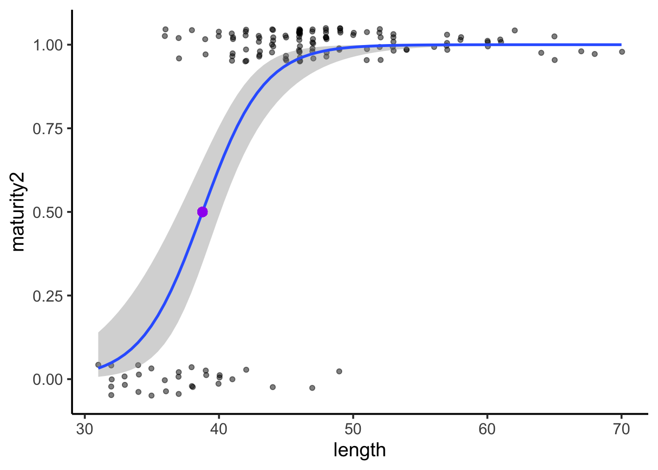
The data and model check out. And remember, if we want to know the inflection point of the model, or the length value where \(p(50)\), we can just divide the negative intercept estimate by the slope estimate. This value, at a length of 39, was added to the above plot in a large purple dot.
# p(50)
-coef(binom.glm)[1]/coef(binom.glm)[2]
## (Intercept)
## 38.76723