Chapter 6 The Linear Model

Understanding what a statistical model is and what statistical estimation is—and knowing the difference—is a critical first step toward analyzing your data. Now that model and estimation are differentiated, we will think about how they work in concert. Before we start in on the actual modeling, let’s get some terms down.

6.1 Terms

Terms used in linear modeling are not standardized, but for the most part they are consistent. Below are some definitions and discussion about terms that will appear in this text, or terms that may be helpful to be aware of.

units – observations or data points, often indexed with \(i\)

\(x\) variable – predictors or independent variables in the model that are included on the right side of the model equation

\(y\) variable – outcome, response, or dependent variable in the model that is typically the lone term on the left side of the model equation

inputs – also called model terms, these are the items on the right side of the model equation; note that while inputs and predictors are often the same thing, they are not technically the same as you can have more inputs in the model than you can have predictors. Predictors refer to the actual independent variables, so for example a model with two predictors could have three inputs if the third input is an interaction terms between the two predictors

residual error – typically the final term on the right side of the model equation that is included to account for any unexplained information

multiple regression – regression including more than one predictor; also refered to as multivariable regression, and not to be confused with multivariate regression (e.g., MANOVA, PCA, etc.)

6.2 Components of the Linear Model

It may be useful to think of the linear model first by the larger pieces of information that comprise it. Here are three ways that you might want to consider the components of the linear model, and they are interchangable so please consider the equation that makes the most sense to you.

response = deterministic + stochastic

outcome = linear predictor + error

result = systematic + chance

As you can see, based on any of the three descriptions, the measured response is on the left side and it is this response that we are trying to understand with predictor variables. On the right side of the equation we have two components: something predicable and something not predicable. The deterministic part is often called the linear predictor and this is where the indepdnent variables and their parameters will live and work. But because the independnent variables will never explain 100% of the response (and if they do, you are not working with a statistical model), we also need to include a term for an unexplained information. This unexplained information is often called residual error.

Coding a linear model into R is not difficult. The lm() function can be used, inside which you specify the left and right side of your model separated by ~. But where is the error term? The error term is estimated, but not specified. Simply by using the lm() function, R knows this is a linear model and that error needs to be accounted for, and the residual error will be included in the model summary.

lm(y ~ x) # where is error term?
lm(y ~ x1 + x2 + x3) # Model inputs are included by simply adding them

6.2.1 The Response Component

In some ways the response component of a linear model is the most straightforward. The response is simply the dependent variable you observed and which you are hypothesizing is a function of the predictor variables you also observed. From a mechanical standpoint, the response variable is simply a vector of observations that are often refered to as \(y\) and can be included in your model as the lone vector of data on the left side of the formula or equation. The response becomes more important when we start to think about its connection to the stochastic component.

6.2.2 The Stochastic Component

As stated above, all statistical models have some error or residual variance that represents observed information that is not accounted for by the predictors or inputs. This stochastic component is directly related to the response variable through a distribution. That is, all data we observe (or the vast majority of data we observe) are thought to have come from some underlying distribution. The heights of 20 people are thought to be observations of some distribution that has the mean and variance of heights from all people. The number of birds we observe on a transect is thought to be a number coming from a distribution of integers that cannot be less than 0. It is critical that we understand how our (response) data were generated and sampled, in order to best inform our deicsion about an associated distribution. The correct underlying distribution for our model will put in place the correct machinery to describe the response variable and capture the residual error. The normal distribution is very common distribution both in the world and in linear modeling, but there are many other distributions to be aware of and which may be at play in your data.

How can we know which distribution is the best for our data? There are a few steps that can be taken to help us confidently arrive at the best distribution for our data.

1. Know your options: It is hard to know which distributions to pick from if you are not familiar with different distribtions that are available. Other than the normal distribution, common distributions include the binomial (and Bernoulli), the Poisson, and beta; however, there are dozens of less common and less used distributions out there.

2. Know how the data were sampled: Often by simply knowing the process that generated the observations, you can be able to focus in on a distribution. For example, if you know your individual observations are successes or failures (which is the same as yes or no and 0 or 1), then you are by definition working with a Bernoulli distribution. Or, if your observations represent counts that cannot be less than 0 and must be integer values, then you might want to consider a Poisson. Working more and more with data and thinking about data in terms of distributions will help build understanding and skills that can help to quickly narrow down on distributions.

3. Know the characteristics of the data: This option is not always helpful, but simply knowing what your data look like might help you arrive at a good guess for a distribution. The challenge with this option is that observed data—especially with small sample sizes—rarely looks like the textbook distributions, in addition to the fact that nearly all distributions have parameters, which means they do not occur in only one shape. While you might want to limit your expectations from plotting your data and understanding its characteristics, you also rarely get into too much trouble from visualizing data and getting a better sense of it.

4. Run and model and explore distributions: For better or worse, models will often run with less than an ideal distribution. This can cause trouble because you could fit a model with the wrong underlying distributional structure. But if you are aware that incorrect models may still be fitted, then you can cautiously use model fitting as an exploratory tool to see how your data work in a model with different distributions.

5. Know that there may not be a perfect answer: The goal is always to get to that one, clear distribution that makes sense and is defensible. However, sometimes we just don’t get there. It could be that while there is one perfect distribution in theory, there are two distributions in practice that work and provide the inferences you need. Further more, for two distributions there may be unique parameter values for each that cause the distributions to approximate each other. In other words, we tend to think of distributions with a characteristic shape, but nearly all distributions have a variety of shapes, and these shapes may overlap with other distributions. Lacking a clear distribution for your data is never desirable, but know that it may something you have to live with—at least for a while.

[IMG]

6.2.2.1 Distributions

While there are dozens of distributions out there, the reality of statistical modeling is that some are much more common than others. Let’s cover 3 of the most common distributions in linear modeling to get familiar with when we might use them.

1. Normal Distribution

Use for continuous data (not restricted to integers)
range from \(-\infty\) to \(\infty\) (your data might not range this much!)
one of the most common distributions
measurements are effected by large number of additive effects (i.e., central limit theorem)
2 parameters: \(\mu\) = mean and \(\sigma\) = variance

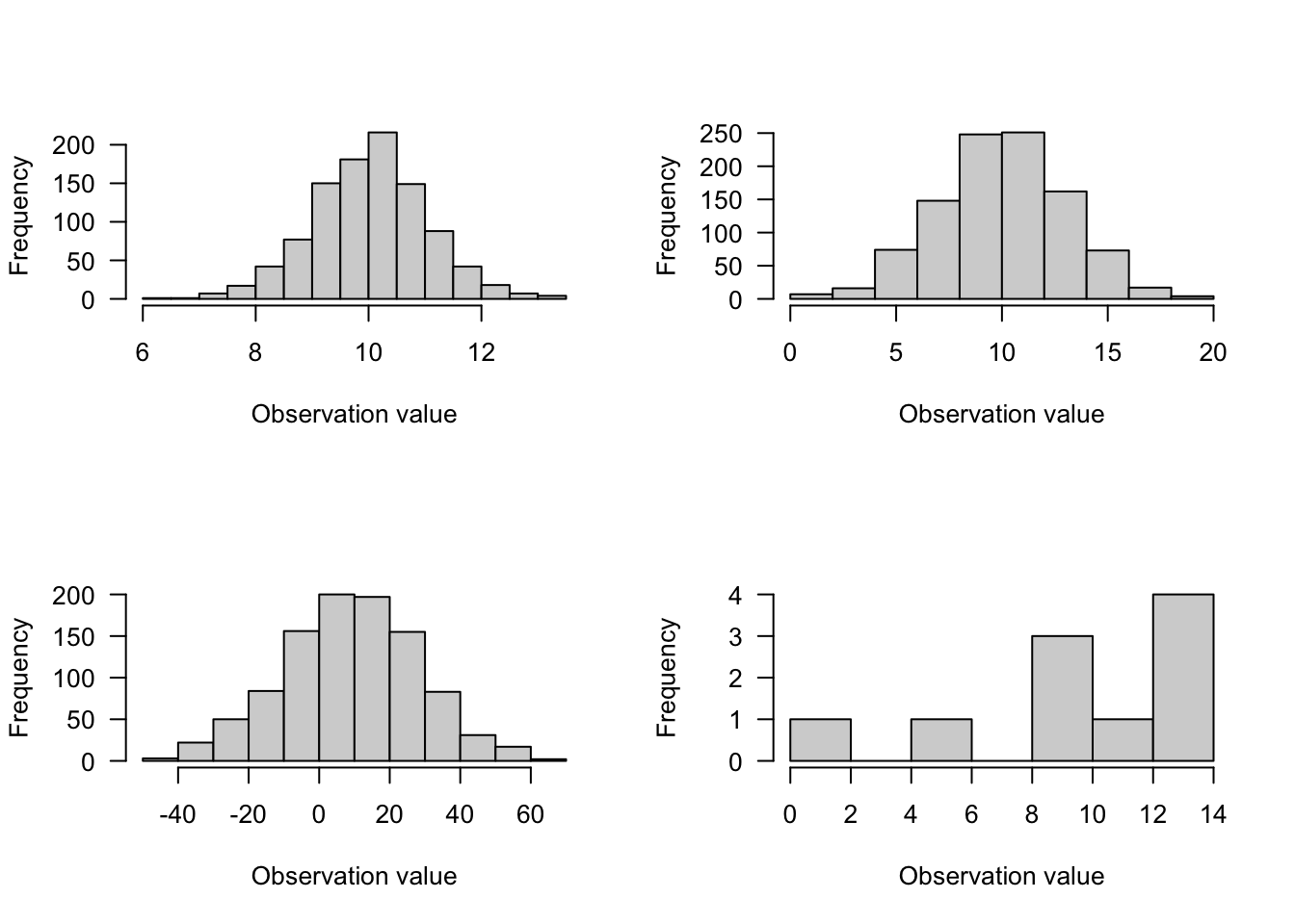
Figure 6.1: Caption

2. Binomial Distribution

Use for discrete integer data in which one observation includes the number of successes out of a total number of trials (maximum number of successes)
2 parameters: \(p\) = success probability and \(N\) = trial sample size
Example, there are 20 individuals enrolled in a class (\(N\)) and 18 attend a given meeting, leading to \(p\) for that trial to be 0.9
The Bernoulli case of the Binomial distribution is when \(N=1\), and the classic example is a coin flip that produces either heads or tails
\(N\) is the upper limit, which differentiates the Binomial from the Poisson distribution
Mean = \(N \times p\)
Variance = \(N \times p \times (1-p)\) (variance is a function of the mean)

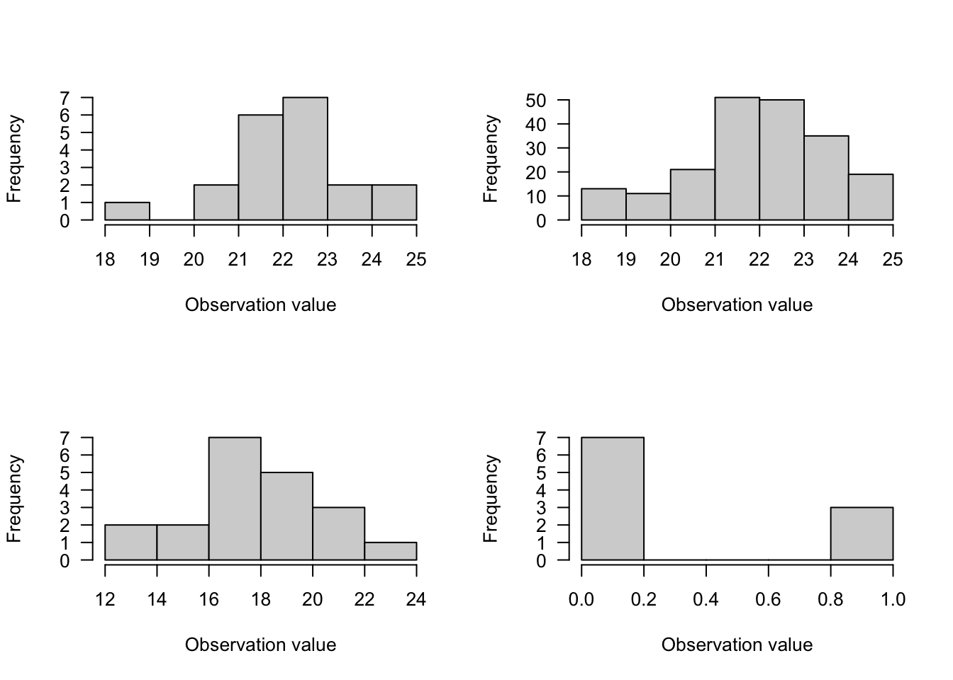
Figure 6.2: Binimial

3. Poisson Distribution

Classic distribution for counts; i.e., integers \(\geq0\) to \(\infty\) (no upper limit)
Useful for number of things in a plot, things that pass a point, things along a transect, etc.
1 parameter: \(\lambda\) = mean = variance
Approximate to Binomial when \(N\) is large and \(p\) is small
Approximate to Normal when \(\lambda\) is large
Modifications exist for zero-inflation and dispersion (e.g., more extreme values than the Poisson distribution would otherwise have)

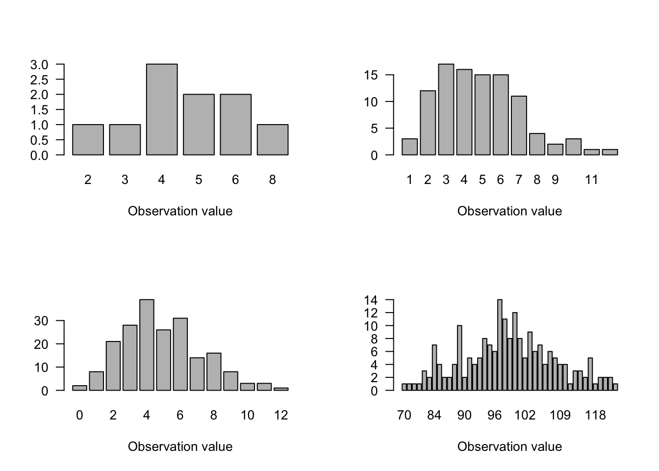
Figure 6.3: Poisson

6.2.3 The Linear Component

Above we have discussed the response component and the accompany probability distributions that might best account for the data in the response component. The remaining part of a linear model is the linear component, which is in some ways is the part of the linear model we most often associate with the model, but also may have more going on than meets the eye. Let’s start with a few facts about the linear component

The linear component is comprised of explanatory variables that have additive effects. Additive effects simply means that predictor effects operate individually, but can be added together. In other words, additive effects are not interactive effects, which is when the effect of one predictor is influenced by the amount or type of another predictor. Although many effects are interactive to some degree and we can add interactive effects to a linear model, let’s start simple and just say that predictor effects are independent of each other.
A linear model does not necessarily mean it has to be a straight line! Yes, the temptation is great to think that “linear” means “line”, and it certainy can mean that. But especially when you get into generalized linear models (GLMs), you will see that a fitted line plotting your model does not need to be a straight line.
Predictors can be continuous and/or categorical. Knowing whether your predictors are continuous or categorical is something your should know for every model you run, but also know that you have flexibility. If you have a continuous predictor, that is typically called regression, with a single continuous predictor called simple linear regression and more than one continuous predictors called multivariable linear regression. Categorical data typically falls into an ANOVA framework, of which there are many flavors. And categorical and continuous predictors can also both be in the same model, as in a case of an ANCOVA, or ANalysis of Co-Variance.
The structure of the linear predictor can be broken down into the design matrix and the parameterization. You can do an awful lot of linear modeling without knowing what the design matrix and parameterization are for your models, so don’t think that this is critical information. However, understanding the design matrix and parameterization may help you understand how the model works and can occasionally be good for troubleshooting. The design matrix and parameterization are very much under the hood of the model, and if running a linear model makes your a driver, knowing about the design matrix and parameterization make you a mechanic.

6.2.3.1 The Design Matrix

Simply put, the design matrix in a linear model is the scaffolding of the model that is used to tell us if an effect is present and how much. The matrix has a number of columns that correspond to the number of fitted parameters. Matrix multiplication is then used with the parameter vector to result in the linear predictor. Make sense? I didn’t think so. Let’s look at a simple model and then look at the design matrix.

# Simulate data for a simple linear regression
set.seed(2)
x <- 2:6
y <- (x-1) + rnorm(5,mean = 0,sd = 0.25)

# summary(lm(y ~ x))
model.matrix(y ~ x)

##   (Intercept) x
## 1           1 2
## 2           1 3
## 3           1 4
## 4           1 5
## 5           1 6
## attr(,"assign")
## [1] 0 1

We can see from the model.matrix() function that we get a matrix with two columns (one for the intercept parameter and one for the slope parameter; the first column is just the row enumeration) and five rows, which corresponds to the number of observations in the dataset. The column for the response and the column for the slope both take the data for y and x, respectively. (Note that the values are rounded in the model matrix, and the column for the response is not technically part of the design matrix, but sometimes it is included for completeness.) The intercept column for each row is equal to 1, wihch is simply an indicator that each observation contributes to the same intercept. Honestly, there is not much to do with this model matrix because we are using a continuous predictor; however, you will see how the design matrix can both change and become important when we have categorical data.

6.3 Linear Models

This next section will simply work through a set of common linear models, approximately from simple to more complex. For each model there will be a short explanation, the statistical formula, the formula in R, and an example. (Note that all residual errors, \(\epsilon_i\) are assumed to be normally distributed with \(\mu=0\) and standard deviation of \(\sigma^2\). Also, we will primarily be running linear models without their summaries, in order that we can just focus on the estimates.)

Let’s code a fake data set in, so that we can use the same dataset for the different models. Let’s call it a fake dataset about fish, where length will be the response variable \(y\), and the other variables may serve as predictors.

weight <- c(16,18,15,27,29,31)
stream <- factor(c(1,1,2,2,3,3))
watershed <- factor(c(1,1,1,2,2,2))
habitat <- factor(c(1,2,3,1,2,3))
length <- c(41,46,37,52,54,60)

6.3.1 Model of the Mean

The model of the mean is probably not a model you would run. However, it is a simplified model that forms the first building block for most regression models. You can think of it as an ANOVA with one group, or as the intercept estimate in a regression. So the model of the mean scores low in real-world application, but high in conceptual importance.

Statistical notation: \(y_i = \mu + \epsilon_i\)
R syntax: lm(length ~ 1)
Application: Infrequent due to simplicity; model building block

In the statistical notation above, \(\mu\) is the parameter we are asking the model to estimate, and \(\epsilon_i\) are the errors represented by each observations distance from \(\mu\).

When we run it in R:

lm(length ~ 1)

## 
## Call:
## lm(formula = length ~ 1)
## 
## Coefficients:
## (Intercept)  
##       48.33

We see that we get an intercept estimate of 48.33. This is the same as if we ran the function mean(length). In essence, this is a model that estimates the mean of one group. So yes, you could run the mean() function to get the same answer, but it remains important to think about how models use the mean(s) in the data, and then compare them or add slopes to them.

By the way, if we ask for the design matrix on this model, it is as simple as possible. The model matrix from R is stimply telling us that each length observation is included (not the actual length measurement, just whether or not we are including it in the model) in the estimate.

model.matrix(length ~ 1)

##   (Intercept)
## 1           1
## 2           1
## 3           1
## 4           1
## 5           1
## 6           1
## attr(,"assign")
## [1] 0

6.3.2 t-test

Let’s say we like the model of the mean, but we have two groups and we want to compare them. The model we would go to would be an ANOVA, but when there are only 2 groups to compare, this special case of ANOVA is called a t-test. Using our fish data, we see we have 2 watersheds, so we might want to use a t-test to compare the lengths of fish between the two watersheds.

Statistical notation: \(y_i = \alpha + \beta \times x_i + \epsilon_i\)
R syntax: lm(length ~ watershed)
Application: Test for the effect of categorical predictor with 2 groups

In the statistical notation above, \(\alpha\) is the first group (often called intercept) and \(\beta\) is the parameter for the effect of the second group. Because \(x_i\) is simply values of 0 or 1 (often called a dummy variable because it is only modeling whether something is included or excluded), \(\beta\) only comes into play when there is a 1 for watershed 2.

When we run it in R:

lm(length ~ watershed)

## 
## Call:
## lm(formula = length ~ watershed)
## 
## Coefficients:
## (Intercept)   watershed2  
##       41.33        14.00

We see two estimates. The first is called intercept and it refers to the first group, in this case watershed1. (Unless specified, groups are always interepted by R either numerically or alphabetically.) The second estimate is called watershed2, and is self-explanatory. In this case, the mean of the first group (intercept) is correctly interpreted as the mean length of fish in watershed 1, and the estimate of 41.33 looks to be about that based on what we know about lengths. However, the mean length of fish in watershed 2 is listed as 14? There are no fish in the data that are even close to a measurement that small, so where does this number come from. The estimate of 14 comes from the fact that 14 needs to be added to the estimate of the first watershed group, therefore 55.33 (or 41.33 + 14) is the mean length of fish in watershed 2.

All of this confusion is happening because R defaults to a certain type of parameterization (remember we introduced that term but didn’t really talk about it?). To step back, there are 2 types of parameterizations: effects parameterization and means parameterization. R defaults to an effects parameterization, which means that the intercept estimate is always the mean of group 1, but it is also the baseline estimate that all other groups need to be combined with. In other words, using an effects parameterization, the estimate for every group after the first one can be thought of as the effect of being in that group compared to group 1. The other type of parameterization is the means parameterization, and a means parameterization simply tells you that each group is given its own mean. In other words, the model has (kind of) already combined the effects and is giving you the group-specific information that does not need to be referenced to any other group. Just to prove it, let’s look at the same t-test as above, but under a means parameterization. Note that a mean parameterization in R’s lm() syntax is easily accomplished by simply subtracting 1 from the right side of the equatio.

lm(length ~ watershed - 1) # Means parameterization of above t-test

## 
## Call:
## lm(formula = length ~ watershed - 1)
## 
## Coefficients:
## watershed1  watershed2  
##      41.33       55.33

Voila. Using the means parameterization, we get the fully baked means. Although this can be confusing, the effects parameterization likely has its roots in historical experimental work, where the first group might have been the control, and it was of interest to see how far from the control mean all the other treatment groups were. Regardless, the good news is that you can change syntax to pick your parameterization, and they both yield the same results; in other words, after you account for the effect parameterization, your estimates will be the same as a means parameterization.

As one last thing, let’s just take a peek at the design matrices from both, because we should see a difference in the design matrices.

# Effect parameterization design matrix
model.matrix(length ~ watershed)

##   (Intercept) watershed2
## 1           1          0
## 2           1          0
## 3           1          0
## 4           1          1
## 5           1          1
## 6           1          1
## attr(,"assign")
## [1] 0 1
## attr(,"contrasts")
## attr(,"contrasts")$watershed
## [1] "contr.treatment"

# Means parameterization design matrix
model.matrix(length ~ watershed - 1)

##   watershed1 watershed2
## 1          1          0
## 2          1          0
## 3          1          0
## 4          0          1
## 5          0          1
## 6          0          1
## attr(,"assign")
## [1] 1 1
## attr(,"contrasts")
## attr(,"contrasts")$watershed
## [1] "contr.treatment"

From these design matrices, you can see how in the effect parameterization all observations are included in the intercept and then only watershed 2 observations are included in the watershed 2 column. However, in the design matrix for the means parameterization, only those length values belonging to specific watersheds are included.

6.3.3 Simple Linear Regression

Moving away from categorical predictors, you will undoubtedly need to run a simple linear regression at some point. Simple linear regression is classically pictured with scatterplot of data points and a best fit line running through them. There are no categories here, just the idea that as \(x\) changes, so does \(y\) (but if it doesn’t change, you can still run the model, it just won’t be significant).

Statistical notation: \(y_i = \alpha + \beta \times x_i + \epsilon_i\)
R syntax: lm(length ~ weight)
Application: Test for the effect of a continuous predictor on the response

In the statistical notation above, \(\alpha\) is the intercept, or the value of y when x=0. Think of it as the value of y when your regression line intercepts 0 on the x-axis. It is important to note that the intercept is very literally interpreted as described above, meaning that for many data sets, a value of x=0 either lies far from the observed data or a value of x=0 has no relevent meaning for your data, and as such, intercept values need to be interpreted with caution. (But not that there are options to scale and transform data that might produce a more meaningful intercept estimate.) \(\beta\) is the parameter for the effect of x, in other words, it is the slope estimate or slope coefficient. A p-value will be one way to tell if your slope is significant, but nonetheless, you can look at a slope value with nothing else and still understand the direction and magnitude of it. Also note how this formula looks identical to the t-test formula, the only change we have made is that x is now continuous and not categorical.

lm(length ~ weight) # Means parameterization of above t-test

## 
## Call:
## lm(formula = length ~ weight)
## 
## Coefficients:
## (Intercept)       weight  
##      21.879        1.167

Our intercept is 21.879, but if we think about what the length of a fish should be when the weight is 0, we quickly understand that this intercept is non-sensical. We need this parameter in the model, but we just need to know that we likely cannot extrapolate from the range of the data. (In this case, it might safe to assume that fish length and weight are linear over the observed data, but over the entire size of a fish, there may be non-linearities.) Our weight estimate of 1.167 is the slope coefficient, and it tells us that for every 1 unit increase in weight, fish length increases by 1.167. Put another way, we know that a slope is the rise over the run, and the run is always 1, so in this case, we could say that fish length increases (rises) 1.167 for every 1 unit increase in weight.

Multivariable regression is accomplished by simply adding one or more continuous predictors to the linear descriptor of the model, and the additional effects are interpreted as additional slopes in the same way we have interpreted the single slope in the above example.

It is also worth noting that when you are modeling continuous data, you do not need to worry about or change your model parameterization.

6.3.4 Analysis of Variance (ANOVA)

The last model we will look at here is the Analysis of variance, but we will only look briefly at it because it is the subject of much deeper investigation in the next chapter. Technically we have already done an ANOVA with two groups, but we called it a t-test. The term ANOVA is most often reserved for models in which there are 3 or more groups of interest. ANOVA is an unbelievably useful and common model with many extensions.

Statistical notation: \(y_i = \alpha + \beta_j \times x_i + \epsilon_i\)
R syntax: lm(length ~ stream)
Application: Test for the effect of 3 or more categorical predictors

Before going into the explanation, it is worth recalling here the distinction between predictors and levels. That is, the predictor is the overall variable, or factor. Within that factor are different categories, or levels. Each level gets its own estimate, but we reserve terms like significance for the overall factor. In other words, if our response variable is number of speeding tickets, we might think that is related to the predictor or factor of car color. But within car color we have 5 levels: black, white, red, yellow, blue. Each of those colors will get it’s own coefficient estimate, yet we still often talk about car color as a significant predictor.

In the statistical notation above, \(\alpha\) is the first group (intercept) and \(\beta\) is the parameter for the additional groups. In this case, I have subscripted \(\beta\) with a j simply to note that there are multiple estimates (levels) within \(\beta\). Another simpler way we could write this model, especially if using a means parameterization, would be \(y_i = \alpha_j \times x_i + \epsilon_i\), which can be interpreted that there are j number of \(\alpha\) estimates and the dummy variable x simply assigns factor levels. The statistical notation for ANOVA can vary widely, so I would encourage you to not get hung up on one way to write the model, but as with any model you run in R, please be prepared to write it in statistical notation.

lm(length ~ stream)

## 
## Call:
## lm(formula = length ~ stream)
## 
## Coefficients:
## (Intercept)      stream2      stream3  
##        43.5          1.0         13.5

You were probably expecting that this would be an effect parameterization, and you were correct. The mean length of fish in stream 1 is 43.5. For the mean lengths of fish in streams 2 and 3, we just take the stream2 and stream3 estimates and combine them with the Intercept.

And just to take a look at the means parameterization:

lm(length ~ stream - 1)

## 
## Call:
## lm(formula = length ~ stream - 1)
## 
## Coefficients:
## stream1  stream2  stream3  
##    43.5     44.5     57.0

It checks out. We will skip running the model.matrix() here because you will more likely just change the parameterization in the model statment than view the design matrix, which you already know how to do.

Finally, the next chapter will go into ANOVA in much more depth, but know that there are several specific functions for ANOVAs, like aov(). You may want to get into the habit of using a specific ANOVA function (instead of lm()), but for now, lm() works and easily shows us the factor level estimates.

6.4 Pre-fitting: Before You Fit a Model

There may be times you quickly want to fit a model to data and not immediately think about assumptions, or, the more you handle data and models the faster your will become with matching the data to the models. However, there is still a series of questions you may want to explore before you fit a model to your data—or at least before you share the results.

It might help to know that pre-fitting and post-fitting activities may inform each other. For example, there may be obvious things to do in the pre-fitting phase, but post-fitting model diagnostics may show that you need to go back and do something else. What this all points to is the iterative nature of model fitting. Even with the same data and model, you may need to iterate several steps to get things in the best shape.

But there are still some actions you can take that are typically handled before you fit your data to a model.

Data transformation. The term transformation can mean a lot of things. What transformation does not mean in this case is taking a non-normal response (e.g., Poisson counts) and transforming it to fit a model that uses an underlying normal distribution. What data transformation means in this case is how we can apply some change to all observations of our data, in the hopes of getting the model to fit a little better.

Linear transformations to normal data result in data that are still normal. For example, if you have a measurement in inches and you want to transform it to centimeters, you have nothing to worry about.
A common transformation is a log-transform, whereby you take the log (log()) of each of your data points. This transformation will help constrain many varieties of clustered or skewed data, and it often helps with the estimation.
Mean-centering data is a simple approach where you subtract the mean of all observations from each observation. This will center your data at 0, which can be useful to help quickly show which values are larger or smaller than the average. Mean centering can also help with model estimation, if your raw observations are large values.
Standardizing data is a step beyond mean centering. When you standaize, you first mean center, and then divide by (typically) 1 or 2 standard deviations. Different standardizations have different meanings, so be sure to check out what the implications are (ADD MORE?)
Lots of transformations are not that useful. For instance, you may find a laundry list of transformations in the literature, many of which are no longer commonly used: square root transform, arcsine transform, etc. Many of these were transformations used in the past to squeeze non-normal data into a shape that looked a bit more normal, but thanks to generalized linear models and other advances, we no longer need to artifically change our response variables.
In general, avoid test of normality. These include the Shapiro-Wilk Test, Anderson-Darling Test, and several others. These tests tend to be very conservative, meaning they will often report that your data is not normally distributed. This has caused many a modeler to either apply a lot of (useless) transformations, or abandon common models for other appraoches. It’s most important to think that your data come from a normal distribution, not exactly that they look like a normal distribution. And what you’ll see later, is that it can be even more important to make sure your model residuals are normally distributed.

Correlated Predictors When you have more than one predictor in a model, you need to make sure they are not too correlated. Having multiple predictors that are telling the same story means that the predictors are competing for the same effect, which can result in questionable or poor coefficient estimates.

There is no exact threshold for how much correlation is too much. Correlations run anywhere between 0 to 1 (or -1 to 0), with correlations closer to 1 meaning the two variables are highly predictive of each other and could be a problem if both in the same model. Although there is no threshold for correlations, around 0.6–0.7 is an amount of correlation that should start to get your attention. Much more than 0.7 and you might expect estimation issues. Below 0.6 and your should be safe.
Common sense should be employed along with correlation. What is meant by this is that a marginal correlation can result in keeping both predictors in the model, or excluding one predictor—and the difference can be common sense or your expert knowledge of the system. A good way to think about this is if the predictors are appraoching a concerning level of correlation and your know that they both represent basically the same hypothesis or mechanism, then the arguement may be to exclude one. Or, if two predicots are approaching a concerning level of correlation, but your expert knowledge can justify that each predictor represents a different hypothesis or mechanism, then it can be justified to keep them both. There is certainly a gray area when it comes to interpreting correlations, so be prepared to justify your decisions.
Correlation matrices are great ways to get quick numerical and visual estimates of correlations between predictors, especially if there are a lot of predictors. There are a lot of packages and functions in R that deal with correlations, but often for pre-fitting diagnostics, you will only need something simple (as shown below).

cor(matrix.object) # correlation values
pairs(matrix.object) # graphical correlation

6.5 Post-fitting: After You Fit a Model

Perhaps even more important than the pre-fitting things to think about is evaluating what comes out of your model. By checking into some simple things, you can greatly increase your confidence in how well the model fits the data and how much confidence you can have in any model estimates.

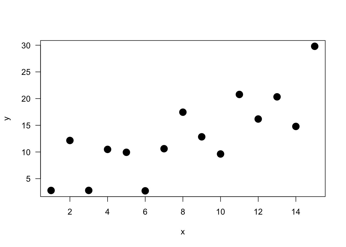
Let’s simulate some data and plot a model, in order to look at the post-fit diagnostics.

n <- 15 # Number of observations
a <- 0 # Intercept
b <- 1.5 # Slope
sigma2 <- 25 # Residual variance
x <- 1:15 # Values of covariate 
set.seed(15)
eps <-rnorm(n, mean=0, sd=sqrt(sigma2))
y <- a + b*x + eps

And a quick visual.

Let’s first run the model.

model5 <- lm(y ~ x)

After running the model, the best thing to do is to check the model summary, which contains a lot of information.

summary(model5)

## 
## Call:
## lm(formula = y ~ x)
## 
## Residuals:
##     Min      1Q  Median      3Q     Max 
## -7.5652 -2.7482 -0.9733  3.3938  7.8172 
## 
## Coefficients:
##             Estimate Std. Error t value Pr(>|t|)    
## (Intercept)    2.494      2.627   0.949 0.359794    
## x              1.299      0.289   4.495 0.000603 ***
## ---
## Signif. codes:  0 '***' 0.001 '**' 0.01 '*' 0.05 '.' 0.1 ' ' 1
## 
## Residual standard error: 4.836 on 13 degrees of freedom
## Multiple R-squared:  0.6085, Adjusted R-squared:  0.5784 
## F-statistic:  20.2 on 1 and 13 DF,  p-value: 0.0006028

Let’s work through all this information.

Model formula: A quick reminder of the model formula that was fit.
Residuals: Residuals are very important as they represent the distance that each observation is from the fitted model. Obviously, we want the fitted model that best describes the data, but there will be some residual error no matter what. What is most important with residuals is that they are normally distributed around 0. If they are not centered around 0, it means the model is over or under predicting too many points. And if the residuals are not normal (i.e., symmetric), it also means something is not being fit well. We don’t need a mean exactly at 0 and perfect symmetry, but we do want to avoid major deviations relative to the data. We want a median residual around 0, and the Min and Max to be relatively the same.
Coefficients: These are simply the parameter estimates. In the model above, the intercept i estimated to be 2.494 and the slope of x is estimated to be 1.299. They will be accompanied by a standard error (Std. Error), which is a measure of uncertainty around the estimate. Finally, the t value is the test statistics that feeds directly into the p-value (Pr(>|t|)). The p-value is likely what you will look at first, but please recall that a p-value is only as good as the model is for the data; in other words, a significant p-value is meaningless or even dangerous if the model is a poor fit for the data.
Significance codes: I suggest to avoid these at all cost. If you want to play by the rules of p-values, then a priori select a significance threshold and that is the only significance threshold that should mean anything. Most people select 0.05.
Residual standard error: This is the standard deviation (spread) of residuals. You may find it useful, but it is not often reported.
Multiple R-squared: % of variance explained by model. Personally, I am not a big user of \(R^2\) values or their variants. The reasons behind this get into a longer discussion that we won’t have, but in general I think there more more effective ways to report on a model. Nevertheless, \(R^2\) is a common model metric and some people will want to know it. Just be reminded that while a higher \(R^2\) is “better”, \(R^2\) always increases with additional model terms
Adjusted R-squared: % of variance explained by model adjusted for more model terms that may not be that explanatory. Basically, this metric is like \(R^2\), but not as liberal as the regular \(R^2\). The formula for the adjusted \(R^2\) is: \(1-(1-R^2)\frac{n-1}{n-p-1}\)
F-statistic: The F-statistic is another test statistic, but one for the model (compared the t statistics which were for individual coefficients). F-statistic tests the null hypothesis that all model coefficients = 0 (ratio of two variances: variance explained by parameters and residual, unexplained variance). You will not typically report an F-statistic in a linear regression model, but you will for an ANOVA.

Let’s go back to the residuals. After you glance over the model summary, you may be satisfied with the model residuals, or you may want to look into them a bit more. If you simply plot the model object (e.g., plot(model5)), you will get a series of 4 diagnostic plots. We will skip that output here because a few of the plots are not diagnostics we are going to get into, and the primary diagnostic—the residual plot—is one we want to be able to manipulate outselves. Again, the residuals are the error, and we expect there to be error—what is more important is that the collective residuals suggest that the model fits the data well without much bias.

We can simply histogram the residuals to see if they are close to being centered over 0 with roughly symmetric (normal) shape.

res <- resid(model5)
hist(res, breaks = 10, las = 1, col = 1, border = "white", xlab = "Residual",main='')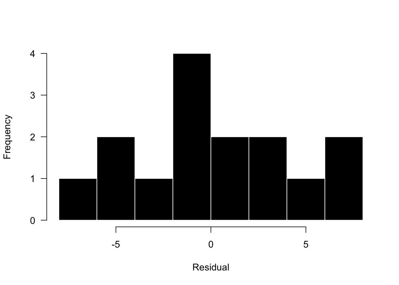

Based on this plot, the residuals look OK. This data set is quite small (n=15), so it would be hard to get a nice symmetric shape, but we see most residuals centered around 0 and the magnitude of positive and negative residuals is about the same. Again, these plots don’t need to look pretty, they just need to not show some bias in the model fitting.

Another way to visualize this data is to plot the residuals as a function of the fitted data. Again, we want to see the residuals spread evenly above and below 0, with no changes in symmetry across the range of fitted values.

res <- resid(model5)
fit <- fitted(model5)
plot(res ~ fit, pch=19, las=1); abline(0,0, col="red")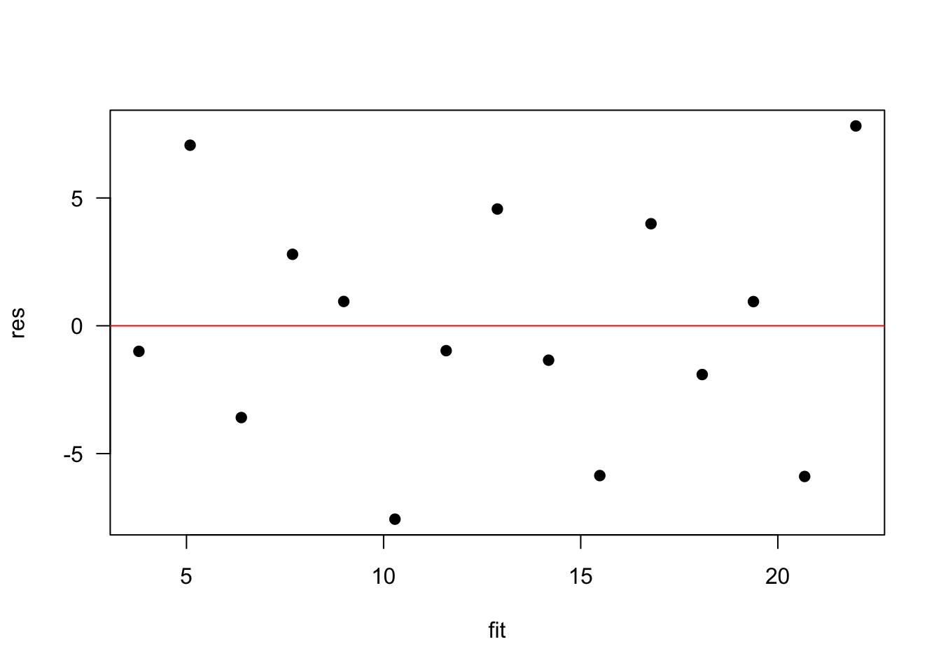

Again, we are dealing with a small sample size, but this looks great.

Ultimately, what we are looking for is often referred to as homoscedasticity, which means residuals are approximately the same. What we don’t want to see is heteroscedasticity, which comes in many forms. Basically, any pattern you can detect in your residuals is evidence that your model may not be fitting your data well across all values of your data. Patterns of heteroscedasticity to look for include fun names like trumpeting and the bow tie, which simply refer to the shape of the residuals when things are not looking good.

(ADD IMAGE?)

6.5.1 Post-hoc Means: Multiple Comparisons

If you run some type of ANOVA and you find that your predictor is significant, you will likely next want to know which factor levels are different from each other. The way to accomplish this is with a multiple comparisons test, also known as a post hoc means test. The underlying issue with multiple comparisons is that as you conduct more statistical comparisons, you run a greater risk of getting false positives. However, if you greatly increase your significance threshold, your significance criteria can become so strict that you error on the other side—you have significant comparisons that go undetected. In a nutshell, all multiple comparisons tests are trying to balance this significance interpretation. Tukey’s Honest Significant Difference (HSD) is one common and pretty versatile multiple comparison method. Please look into others and know which one you are using, and why (citation).

6.6 ANCOVA: Analysis of Co-Variance

Many of the models we have discussed so far are fairly simple and you may be thinking that you would like a model that combines the elements of regression and a continuous predictor with a categorical predictor (as in ANOVA). This is called an ANCOVA or an analysis of covariance. Think of it as an ANOVA that controls for the effect of a continuous co-variate that is often of less interest. ANCOVA can increase the power to detect differences by reducing the within group variances. Another important consideration for ANCOVA is an interaction term. An interaction term in an ANCOVA can often be evaluated early as diagnostic to understand the relationship between the continuous and categorical predictors, and the significance of the interaction term may determine how you proceed. A significant interaction term between your continuous and categorical predictor indicates that the effect of the continuous co-variate on the response depends on the level of the categorical factor. There are a number of different interpretations on how to handle this; however, it is commonly recommended that if the interaction is not significant you do not have to worry about the continuous co-variate providing different effects and interpretation on different factor levels. Thus, you can safely remove the interaction term and simply run your model with the main effects. However, if the interaction term is significant you’ll need to consider the implications. First off it may be hard to interpret the main effects of the model when the interaction term tells us that the main effects are dependent on each other and thus not necessarily able to be interpreted in isolation. In other words, a significant interaction tells us the effect of the continuous predictor is different on different factor levels of the categorical factor. As such, what does the continuous predictor mean without the context of the specific factor levels?

6.6.1 Interactions

It should be noted that interactions can be used in a wide variety of linear models and are not confined to ANCOVA models. (It’s just that many of us first encounter interactions in the context of an ANCOVA, which make their association a reasonable place to introduce interactions.)

The main idea behind an interaction is that the effect of \(x_1\) on \(y\) depends on the level or quantity of \(x_2\). In an ANCOVA,\(x_1\) is the continuous predictor and \(x_2\) is our categorical factor; however, both \(x_1\) and \(x_2\) can be either variable type. It’s often advisable to have a reason or hypothesis for the interaction. In other words it is not advisable to simply interact terms just because you can. Interactions get much more complex than we were able to cover in this text but they can be a powerful statistical tool and you are encouraged to look into them more as needed. A few cautions: First, you will likely need and increased sample size as you run interactions (citation). Second, it’s also advised to avoid 3-way interactions, unless you have a strong motivation (i.e., hypothesis) for doing so.

A statistical equation for a linear model with two main effects and one interaction (the product of the two main effects) might look like:

\(y_i = \alpha + \beta_1x_1 + \beta_2x_2 + \beta_3x_1x_2 + \epsilon_i\)

Syntax for interactions in R can take use the colon (:) if you want only the interactive effect or the asterisk (*) indicating multiplication if you want both the interactive effect and both main effects.

# LM with two main effects (no interaction)
lm(y ~ x1 + x2)

# LM with two main effects and interaction
lm(y ~ x1 * x2)

# Same as above
lm(y ~ x1 + x2 + x1:x2)

# LM with interaction and no main effects
lm(y ~ x1:x2)