Chapter 7 Understanding ANOVA in R
7.1 Introduction
ANOVA (or AOV) is short for ANalysis Of VAriance. ANOVA is one of the most basic yet powerful statistical models you have at your disopsal. While it is commonly used for categorical data, because ANOVA is a type of linear model it can be modified to include continuous data. Although ANOVA is relatively simple compared to many statistical models, there are still some ins and outs and what-have-yous to consider. This tutorial explores both the features and functions of ANOVA as handled by R.
Like any statistical routine, ANOVA also comes with it’s own set of vocabulary. I can’t promise that I will cover it all, but it should help to know that ANOVAs are typically referred to as 1-way and 2-way, which is just a way of saying how many factors are being examined in the model. (ANOVAs can be 3-way or more, but these are less common or end up with different names.) A factor is the categorical variable that you are evaluating, and the different categories within the factor are often called levels or groups. This language is somewhat flexible, just don’t call a specific level a factor. Of course, ANOVAs can have many more than 2 factors, but as with any model, there are costs and benefits as models increase in complexity. We can add a continuous covariate to our model, which results in a hybrid ANOVA and linear model that is called ANCOVA—an ANalysis Of COVAriance.
7.2 ANOVA Mechanics
To truly understand how ANOVA works, you would need to consult a proper statistical text—this text is more of a working man’s version of using statistical tools. However, I will take a few lines here to provide a broad overview of how ANOVA works. To start, let’s think of the name: analysis of variance. So in its roughest form, ANOVA analyzes the variance in the data to look for differences. It does this by considering two sources of variance, the between-group variance and the within-group variance. The between-group variation is calculated by comparing the mean of each group with the overall mean of the data—so individual data points don’t matter quite as much as just comparing group means. The within-group variation is the variation of each observation from its group mean. For both types of variance, a sums of squares (SS) is the numerical metric used to quantify them and this metric simply sums the distances of each point to the mean. The ratio of these SS (between SS divided by within SS) results in an F-statistic, which is the test statistic for ANOVA. The F-statistic is then combined with the degrees of freedom (df) to arrive at a p-value, which, to be honest is what we are all here for. Another way to think of it is that small p-values come from large F-statistics, and large F-statistics suggest that the between group variance is much larger than the within-group variance. So when the differences in group means is larger and yet the groups are not that variable, we tend to have significant factors in our ANOVAs.
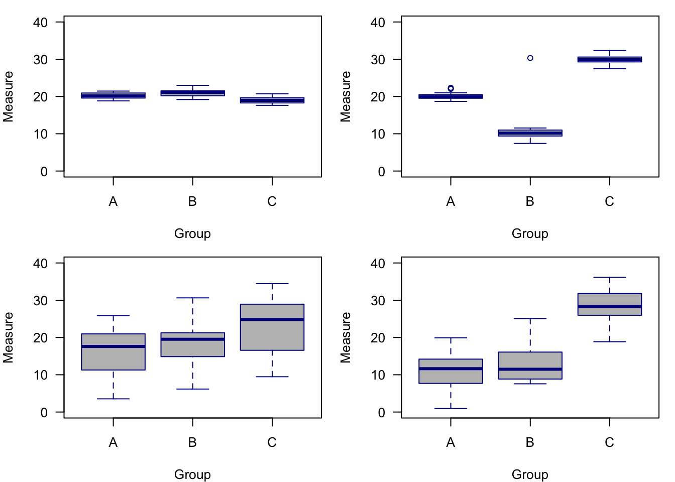
Figure 7.1: Examples of different sums of squares. The top left panel shows little within-group variance and little between-group variance. The top right panel shows little within-group variance, but high among-group variance. The lower left panel shows high within-group variance but low among-group variance. The lower right panel shows high within-group variance and high among group-variance.
7.3 Generate ANOVA Data
Let’s start with a basic example of a categorical dataset. Consider the maximum size of 4 fish each from 3 populations (n=12). We want to use a model that will help us examine the question of whether the mean maximum fish size differs among populations.
size <- c(3,4,5,6,4,5,6,7,7,8,9,10)
pop <- c("A","A","A","A","B","B","B","B","C","C","C","C")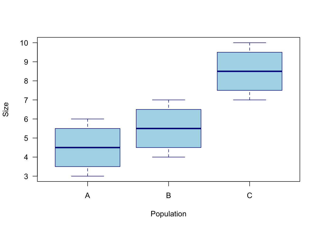
Figure 7.2: Visual of fake dataset looking at the value of maximum fish sizes for three different populations.
Using an ANOVA model will answer the question whether any group means differ from another. There are a few important things in that statement. Specifically, ANOVA will only tell us if one or more group(s) differ from another—it will not tell us which groups differ. We may visualize the data and think we know, but please hold back from drawing conclusions about group differences based only on an ANOVA and/or a figure.
7.4 ANOVA using lm()
We can run our ANOVA in R using different functions. The most basic and common functions we can use are aov() and lm(). Note that there are other ANOVA functions available, but aov() and lm() are build into R and will be the functions we start with.
Because ANOVA is a type of linear model, we can use the lm() function. Let’s see what lm() produces for our fish size analysis.
lm.model <- lm(size ~ pop)
summary(lm.model)
##
## Call:
## lm(formula = size ~ pop)
##
## Residuals:
## Min 1Q Median 3Q Max
## -1.50 -0.75 0.00 0.75 1.50
##
## Coefficients:
## Estimate Std. Error t value Pr(>|t|)
## (Intercept) 4.5000 0.6455 6.971 6.53e-05 ***
## popB 1.0000 0.9129 1.095 0.30177
## popC 4.0000 0.9129 4.382 0.00177 **
## ---
## Signif. codes: 0 '***' 0.001 '**' 0.01 '*' 0.05 '.' 0.1 ' ' 1
##
## Residual standard error: 1.291 on 9 degrees of freedom
## Multiple R-squared: 0.698, Adjusted R-squared: 0.6309
## F-statistic: 10.4 on 2 and 9 DF, p-value: 0.004572First we see our model call that simply reminds us of the model we fit. Next we see our residuals that we may want to evaluate for model fit. Assuming the model fit is reasonable, we can now look at some of the statistics from the ANOVA. Under coefficients, we see three categories, although popA is missing and (Intercept) is listed as the first coefficent. This is because the function defaults to an effects parameterization, whereby the first categorical group, popA, is the reference or baseline group and is called the intercept. The coefficient estimate for that group is the first group’s mean, but the coefficients for the other groups represent the effect of being in that group, hence the effect parameterization. The way to get the group coefficients for all groups after the first group is to add the estimate of the intercept (first group) to each of the other groups. So in the example above popA has a mean maximum size of 4.5, while the mean maximum size of popB is 5.5, the combination of 4.5 and 1. It is advisable to ignore the test statistics and p-values for the individual coefficients as there are better ways to examine them.
With all that being said about the coefficients, you may want to skip immediately looking at the coefficients and look to the bottom of the model summary where the F-statistic is reported along with the p-value on that F-statistic. The F-statistic is the test statistic for ANOVA and is a combination of the sums of squares described above. The associated p-value can help provide a significance interepretation on the F-statistic. That is, a p-value \(< 0.05\) tells us that at least one group mean differs from another at the \(\alpha = 0.05\) level of significance. What does all this mean? It means if you run your ANOVA and skip to the p-value, a p-value \(>0.05\) suggests no group means differ from each other and you may be done with that model. If the p-value \(<0.05\), then you have at least one group that differs from the other(s) and additional steps need to be taken to quantify those differences.
7.5 ANOVA using aov()
A simple and perhaps perferred1 way to do an ANOVA in R is to use the aov() function. Let’s try that function on the same model we examined above with the lm() function.
aov.model <- aov(size ~ pop)
summary(aov.model)
## Df Sum Sq Mean Sq F value Pr(>F)
## pop 2 34.67 17.333 10.4 0.00457 **
## Residuals 9 15.00 1.667
## ---
## Signif. codes: 0 '***' 0.001 '**' 0.01 '*' 0.05 '.' 0.1 ' ' 1It is worth noting that your categorical variable in the aov() needs to be a factor. For example, you may have categorical groups labeled 1–10, but of those labels are numeric or integeter in the eyes of R, then they won’t work in aov(). Fortunately, the as.factor() wrapper usually does the trick.
Back to the aov() output. First, notice it is greatly reduced compared to the lm() output. This is because aov() just reports on the ANOVA-specific information, which again is somewhat basic to start. We can clearly see the F-statistic along with the p-value—and we are happy to see that they match the F-statistic and p-value from the lm output. We get a little different information in the aov() function, however. We get degrees of freedom, sum of squares and mean squares, which you may want for your model reporting.
We may want the ANOVA coefficients, which are not included in the summary. Fortunatly, those can easily be had by subsetting the model object.
aov.model$coefficients## (Intercept) popB popC
## 4.5 1.0 4.0And again, they match the lm output, which is reassuring to see and they are in the effect parameterization. Also note that despite the relatively basic model summary for aov, there is a lot of information in the model object, much of it beyond what the basic modeler will need.
We have an ANOVA that has detected a significant effect of the factor, which in this case is population. We know this because the p-value \(<0.05\). We could simply report this and call it done, but chances are you or your audience will want to know which groups differ from each other. Recall that we cannot just infer this from a visual of the data, but fortunatly there are statistical tests to help us understand the group differences.
7.6 Multiple Comparisons
Often called post-hoc comparisons or means comparisons, multiple comparisons is the analysis after ANOVA that helps us quantify the differences between groups in order to determine which groups significantly differ from each other. There are many versions of multiple comparisons test, which range from anti-conservative (more likely to detect siginficant differences) to conservative (less likely to detect significant differences). It behooves the modeler to know which multiple comparisons test(s) are accepted within their discipline; however, here we will cover a very common test called the Tukey’s Honest Significant Differences (HSD).
Tukey’s HSD requires an aov object on which it runs its procedure—so don’t do an ANOVA in lm and then try to use it in a Tukey test. The Tukey HSD procedure will run a pairwise comparison of all possible combinations of groups and test these pairs for significant differences between their means, all while adjusting the p-value to a higher threshold for significance in order to compensate for the fact that many statistical tests are being performed and the chance for a false positive increases with increasing numbers of tests.
TukeyHSD(aov.model)## Tukey multiple comparisons of means
## 95% family-wise confidence level
##
## Fit: aov(formula = size ~ pop)
##
## $pop
## diff lwr upr p adj
## B-A 1 -1.5487408 3.548741 0.5402482
## C-A 4 1.4512592 6.548741 0.0045122
## C-B 3 0.4512592 5.548741 0.0231730Fortunately, with our example we only have 3 different pairwise comparisons to evaluate; however, know that when you have a high number of factor levels, you will get a lot of pairwise comparisons to consider.
Looking at the Tukey HSD output, the first column is the pairwise comparisons, in this case the two populations that are being compared. After that, the diff column provides an estimate of the mean difference between the groups, and the lwr and upr columns give us the lower and upper bound of the confidence interval on the difference. If the confidence interval overlaps 0, we have a non-significant comparison (i.e., the difference is not significantly different from 0), and if the confidence interval does not overlap 0, we do have evidence for a significant difference between groups. In addition to looking at the confidence intervals, the p-value for the individual comparison will also provide interpretation on any significant difference.
Based on p-values \(<0.05\) we have two groups combinations that differ: C-A and C-B. This does largely match our visual from earlier, where population C showed a much larger value than populations A and B. We also see that there is no evidence that populations A and B differ—so any visual differences we may have noticed are not statistically significant. Stepping back for a minute, the TukeyHSD output also gives us other information.
Although there are many ways to visualize multiple comparisons and I would encourage you to be creative, know that your can simply plot the TukeyHSD() function for a reasonable figure that might get you started.
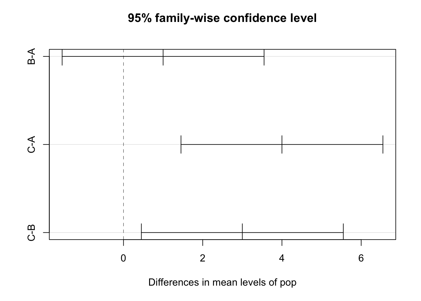
Figure 7.3: Visual of Tukey’s HSD pairwise comparisons available through by plotting the TukeyHSD function.
7.7 Means Parameterization of ANOVA
You may be familiar with the means parameterization of linear models. Means parameterizations basically mean that the model estimates coefficients that reflect the group means, and not the effect of a group compared to the referenece group (intercept). ANOVA may be a good place to consider a means parameterization if you are interested in the group means and don’t like simple math. However, please know that a means parameterization of an ANOVA model does change the hypothesis of what the model expects to be doing, and therefore the p-values are likely also to be changed. Let’s explore.
To means parameterize our aov model, we need to add -1 to the model formula. Think of this as basically telling the model to subtract the intercept or reference group.
aov.model <- aov(size ~ pop - 1)
summary(aov.model)
## Df Sum Sq Mean Sq F value Pr(>F)
## pop 3 491 163.67 98.2 3.4e-07 ***
## Residuals 9 15 1.67
## ---
## Signif. codes: 0 '***' 0.001 '**' 0.01 '*' 0.05 '.' 0.1 ' ' 1This output is quite a bit different from the effects parameterization. You may notice that the Sum Sq and Mean Sq are much larger. How can this be—the data did not change? What a means parameterization is doing is setting each group mean to 0, and if your data are not close to 0, this can result in some very large estimates of error. We also see a large F-statistic and miniscule p-value. This means parameterized ANOVA is testing the hypothesis that the means are different from 0, which of course they are. If you look at the model coefficients, you will see what you expect from a means parameteriztion, but please be aware of the different interpretation of the model summary.
Just for the sake of exploring, let’s see what happens when we mean-center our data and then run it in a means parameterized ANOVA. Mean-centering applies a simple transformation that subtracts the mean value from all of our data and results in the data being centered over 0. We are just shifting the numberline under the data, so this is a safe and simple transformation. In theory, we should expect our errors to be greatly reduced and to have a smaller F-statistic and larger p-value.
size.c <- size - mean(size)
aov.model <- aov(size.c ~ pop - 1)
summary(aov.model)
## Df Sum Sq Mean Sq F value Pr(>F)
## pop 3 34.67 11.556 6.933 0.0103 *
## Residuals 9 15.00 1.667
## ---
## Signif. codes: 0 '***' 0.001 '**' 0.01 '*' 0.05 '.' 0.1 ' ' 1As expected, our errors are greatly reduced, our F-statistic smaller, and our p-value much larger. Note that the model is still siginficant and doesn’t match our default effects parameterization—which we don’t expect it to—but this mean-centered example simply affirms how ANOVA works on our data.
I say preferred because
aovis designed for ANOVA where aslmsimply has the ability to run an ANOVA. The output fromaovis also a bit more straightforward, and therefore tends to reduce the chance of interpreting something that may not be relevant, like a p-value on the effect coefficient of a factor level.↩︎