Chapter 9 Random Effects
9.1 Introduction
9.1.1 A note on terminology
Before we get into what random effects are it’s worth mentioning that the random effects topic introduces a lot of new vocabulary, much of which can be confusing even to those comfortable with random effects. Random effects are really at the core of what makes a hierarchical model; however, the term hierarchical can mean a lot of things to a lot of different people. An explicit hierarchical model (Royl and Dorazio 2008) would be something like a state space model in which the observation in system are modeled separately. Hierarchical models are sometimes also referred to as multi-level models, which may not necessarily be a state space model, but models in which the random effects coefficients are then modeled in the subsequent level of the model (Gelman and Hill 2006). Regardless of the confusing vocabulary, it’s worth knowing that the terms hierarchical, model-multi level model, random effects model, mixed effects model, and varying coefficients model (some sometimes other terms) all may be used to mean similar or different models. When in doubt, seek details on what the model is trying to do, not just what the model is called. This text will adopt the simple terminology of a mixed model when both random effect(s) and fixed effect(s) are present in the model, or a random effects model when all model effects are random effects.
As challenging as it may be to pin down the correct vocabulary for random effects what is more clear is that hierarchy exists in nature and once you understand random effects and the hierarchy they can describe, you’re likely to see them in numerous situations. Nature is hierarchical—why shouldn’t our models be? You may already be thinking about streams nested in the watershed, species grouped in a family, repeated measurements taken on one experimental unit, and numerous other cases of where observations or groups tend to be clustered within some common unit. These are all situations in which a random affect is very likely to improve your ability to model the system.
Ultimately the application of random effects to create a mixed- or random effects model is all done to capture more realism in the system we are seeking to describe with our models. Specifically we wouldd like to better account for correlated structures and uncertainty. Correlated structures may come from the fact that you have multiple observations within a common unit or otherwise lack complete independence across your observations. Not using hierarchical models also comes with a caution: while all models are to some degree incorrect, inaccurate estimation of factor levels or pooling dissimilar information may extend the degree to which the model is inaccurate thus making the results incorrect or even worse—misleading.
9.2 Variance
In order to understand mixed- and random effects models we need to understand random effects, and to understand random effects we need to understand variance. We often need to think more about where the variance in our system is showing up in our model or how our model is handling the variance that we know will be there. Historically variance was seen as noise and distraction and the objective was to remove or minimize all possible variance. Variance was often seen as a nuisance parameter. However “20th century science came to view the universe as statistical rather than clockwork and variation is signal rather than noise.” (Leslite and Little 2003). There has been somewhat of a move to not try to scrub our models of all variance, but rather to find the right home for the variance. In other words there can be information in the variance. Variance is ubiquitous but understanding what part of the system holds what proportions of the variance can be very helpful to our understanding the systems we seek to model. We are familiar with the residual variance from our linear models, but might that residual variance be better attributed to within a group? Or between a group?
9.3 Fixed and random effects
One way to deal with variance concerns how you treat your categorical factors in your model. Recall a factor is a categorical predictor that has two or more levels. We have encountered factors before when talking about t-tests or ANOVAs. However, up to this point we have only talked about fixed factors, and a fixed versus a random factor addresses how the factor levels interact with each other and what assumptions and information can come from the factor levels. A fixed factor assumes that the levels are separate, independent, and not similar. A random effect assumes the levels come from a distribution of levels and while they each have their own independent estimates, they are assumed to be related and exchangeable.
9.3.1 Fixed Effects
Fixed effects are probably more common than random effects, at least in their use (but perhaps not in reality). Fixed effects estimate separate levels with no relationship assumed between the levels. For example in a model with a fixed effect for fish sex you would get an estimate for male and then estimate for female separately. There is no assumed relationship between these two levels. This means we cannot infer what happens between the levels even when it may be obvious. Fixed effects also assume a common variance known as homoscedasticity. Post hoc adjustments are needed to do pairwise comparisons of the different factor levels, should we find reason that they differ.
Another simple example of a fixed effect might be thinking about the fixed effect of a treatment drug on a health response. The predictor drug may be a fixed factor with 4 levels, representing 4 different drugs—a placebo, Drug A, Drug B, and Drug C. In this case, we might design an experiment that could be analyzed with an ANOVA and as we test for the effect of the different drug levels, we want them to be independent of each other—meaning the effect of Drug A compared to Drug B should only include information about those two groups. We don’t want information or even the assumption of non-independence to infiltrate the groups we want to compare. Again, fixed effects are the default effects that we all learn as we begin to learn statistical concepts and fixed effects are the default effects in functions like lm() and aov().
9.3.2 Random Effects
Random effects are less commonly used but perhaps more commonly encountered in nature. In a random effect each level can be thought of as a random variable from an underlying process or distribution. Estimation of random effects provides inference about the specific levels (similar to a fixed effect), but also population level information and thus absent levels. This is often referred to as exchangeability, which is the idea that the given levels in a random effect are not separate and independent but really representative levels from in larger collection of levels, which may not even be observed.
A random effect is another way to think about an effect that may be in your model. Admittedly, the term random can be misleading as there there is nothing inherently random about random effects. The way to think about random effects is that each level of the effect could be considered a draw from a random variable. In other words, the levels or groups in a random effect can be conceptualized as a sample of levels from a larger population of levels—some of which may not be represented in the model. An simple example of a random effect in a model might be the response of shrub height predicted by the categorical effect of forest type. More specifically, we might think that although our dataset only includes 4 different forest types in which we collected data—bottomland hardwood, longleaf pine, Aspen-Birch, and Redwood forest—that the four forest types we observed are just 4 samples from a larger collection or distribution of forest types out there.
Consider a simple example where A is a fixed effect and B is a random effect. If A has 10 levels, then inferences or estimates are only applicable to those 10 levels. If B has 10 levels they are assumed to represent an infinite number of levels and our inferences therefore extend beyond the data and can even be used predictively. To further develop this example let’s consider a model where we have an effect of person and there are 10 people ( 10 levels ) in our model. Each of these 10 people are part of a study to measure how many hours per week they exercise over a 5-week period. Data (n=50) are measured such that each person has five observations which represents their summed hourly exercise for each of the five weeks of the study. If we treat people as a fixed effect it means we can only estimate the means of the 10 individuals. A fixed effect model also assumes that each of the individuals has a common variance around their exercising that variance is the same or similar to everyone else in the study. If individuals are random effects that means we can estimate the mean and variance of our participants and make a reasonable prediction about others that were not enrolled in this study. We also know that because we repeated our measurements on individuals, the number of hours exercised within a given individual is much likely to be similar than the observations compared to someone else. In this case a random effect would be justified.
9.4 When are random effects appropriate?
Ultimately you can find your own support for whether or not to use random effects. This means it is wise to understand random effects so that you’re able to make your own decisions and support them in a defensible way. Gelman and Hill (2006) note that “the statistical literature is full of confusing and contradictory advice.” They also said “you should always use random effects.” I have adopted that recommendation but replaced the word use with the word consider–you should always consider random effects. There are several reasons why random effects extract more information from your data and better allocate the variance in your model. The built-in safety is that if you have no real group level information or random effects at play, the random effects estimates will essentially revert back to fixed effects estimates.
Perhaps it is clearer to understand when you might not want to use random effects. You might not want to use random effects when your numbr of factor levels is very low. There’s no firm rule as to what the minimum number of factor levels should be for random effect and really you can use any factor that has two or more levels. However it is commonly reported that you may want five or more factor levels for a random effect in order to really benefit from what the random effect can do. Another case in which you may not want to random effect is when you don’t want your factor levels to inform each other or you don’t assume that your factor levels come from a common distribution. As noted above, male and female is not only a factor with only two levels but oftentimes we want male and female information estimated separately and we’re not necessarily assuming that males and females come from a population of sexes in which there is an infinite number and we’re interested in an average.
9.4.1 Partial pooling and shrinkage
This text will not get deep into the mechanics of partial pooling, but it is worth noting that random effect estimates are a function of the group level information as well as the overall (grand) mean of the random effect. Group levels with low sample size and/or poor information (i.e., no strong relationship) are more strongly influenced by the grand mean, which is serving to add information to an otherwise poorly-estimated group. However, a group with a large sample size and/or strong information (i.e., a strong relationship) will have very little influence of the grand mean and largely reflect the information contained entirely within the group. This process is called partial pooling (as opposed to no pooling where no effect is considered or total pooling where separate models are run for the separate groups). Partial pooling results in the phenemenon known as shrinkage, which refers to the group-level estimates being shrink toward the mean. What does all this mean? If you use a random effect you should be prepared for your factor levels to have some influence from the overall mean of all levels. With a good, clear signal in each group, you won’t see much influence of the overal mean, but you will with small groups or those witout much signal.
9.5 PLD Example
Let’s consider an extended example to think about random effects. This will be the planktonic larval duration (PLD) example from O’Connor et al (2007). We know that temperature is important for developing organisms. In marine species temperature is an important link to growth and thus time spent as a planktonic larvae can have effects on mortality and other important population regulating processes. Historically these relationships have looked at the between species comparisons but not the within species comparisons. It may be very important to consider both within and between species aspects of this data in order to understand where the variability lies and how best to model the data.
Let’s first look at the overall data plotted without any group information. (Note that the response and predictor were log transformed to improve model fit.) A total of 214 observations are included in the data.
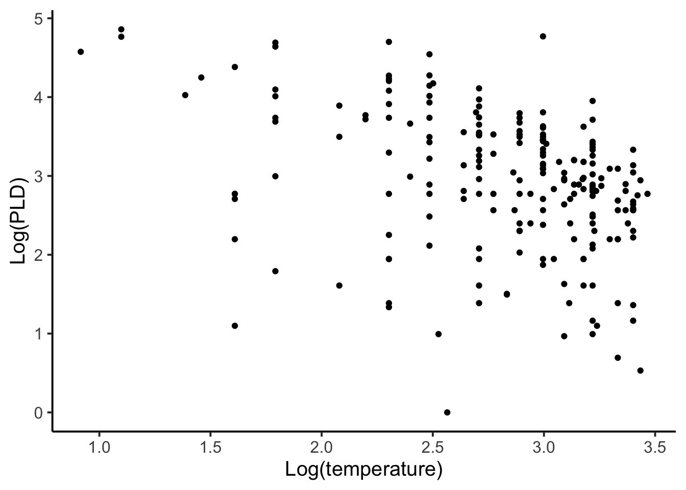
When first seeing this data and thinking about modeling it we might entertain two options. The first option would be to aggregate or to distill each species into one observation. In this case our total sample size goes from 214 down to 72, which is the number of unique species in the data. This approach also ignores within-species variation, which is dangerous because it may be a large part of the overall variance and thus result in a loss of information and power. When aggregating, each sample becomes a subsample. So in a way we’re not actually modeling any of the observed data, but rather we are modeling means or averages of the data.
A second approach to modeling this data may be to disaggregate it. By disaggregating it all observations would be used but no species factor would be included (similar to the first PLD figure). Each observation is considered an independent replicate sample, which we know is not likely to be true because measurements within species are more likely to be similar than compared to other species. We also know that species with larger sample sizes would contribute disproportionately to the coefficients even though there groups are not being explicitly included. For example, if we had a species for which there were a large number of observations and a species in which there were only one observation, under a disaggregated approach the species with a large number of observations would have a disproportionate influence on the outcome of a disaggregated model.
Let’s compare the model output for the aggregated and disaggregated approaches.
| Approach | Intercept | Slope | p-value |
|---|---|---|---|
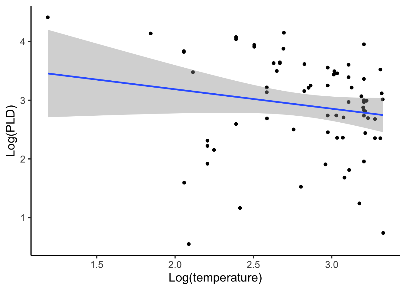
| Aggregated | 3.85 (2.59, 5.10) | -0.33 (-0.77, 0.11) | 0.22 |
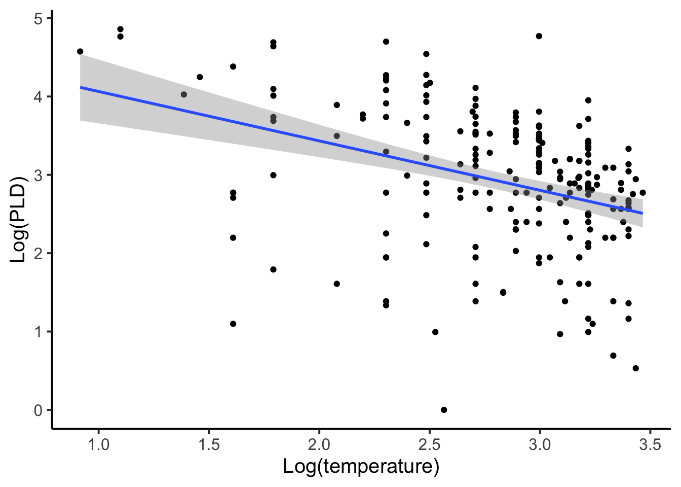
| Disaggregated | 4.69 (4.08, 5.31) | -0.63 (-0.85, -0.42) | < 0.001 |
We can see from the above table that the aggregated approach has less statistical power, meaning that it has wider confidence intervals and a non-significant effect of slope. The disaggregated model has larger coefficients, tighter confidence intervals, and statistical significance. Where did this significance come from?
At this point you may be questioning both the aggregated and disaggregated appraoches. Both have their flaws. In fact, this data is an excellent candidate for a random effect. We expect the overall temperature and PLD relationship to be similar among species, but not the same. We also know there are more than 72 species in the ocean, and as such species are not necessarily great fixed effects.
9.6 Types of models with random effects
Let’s pause on the PLD data and now discuss what specific types of mixed- and random effects models we have readily available. The figure below shows common linear regression models ranging from a conventional fixed effects model to a fully random effects model.
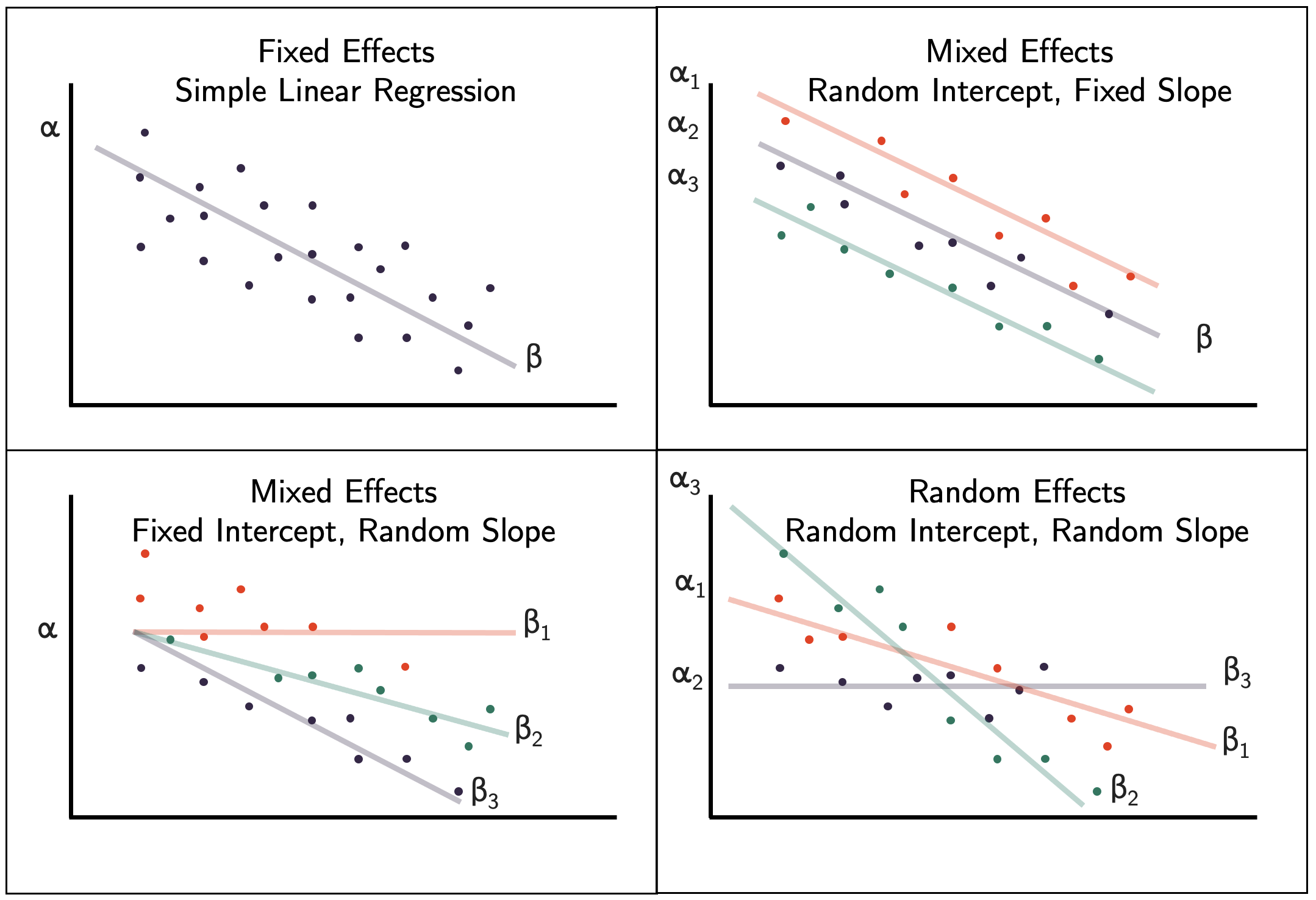
Figure 9.1: Fixed effect, mixed effects, and random effects linear regression models.
We know the fixed effects model, so that model is just a reference. Let’s think about the mixed effects models first.
9.6.1 Mixed effects models
Mixed effects models have exactly that—mixed effects including both fixed and random effects. The first mixed effect model we might consider is one that has a random effect for the intercept and fixed slope. This means each group in the model gets its own intercept estimate, but has a common slope.
Let’s bring the PLD data back for some model fitting. For the sake of simplicity and space, let’s subset the pld data down to just phylum Mollusca, which still includes 16 species, but helps us focus on specific groups (and avoid 72 panels in a plot).
mol <- filter(pld, phylum == "Mollusca")9.6.1.1 Random intercept, fixed slope model
The first model we will examine is the mixed effects model with a random intercept and fixed slope. Let’s first look at the species-specific plots to have a baseline of what each species relationship looks like when fitted to its own data.
ggplot(mol, aes(y = l.pld, x = l.temp)) +
  geom_point() +
  xlab("Log(temperature)") +
  ylab("Log(PLD)") +
  theme_classic(base_size = 15) +
  stat_smooth(method = "lm", formula = 'y ~ x', se=F,fullrange = T) +
  facet_wrap(~species)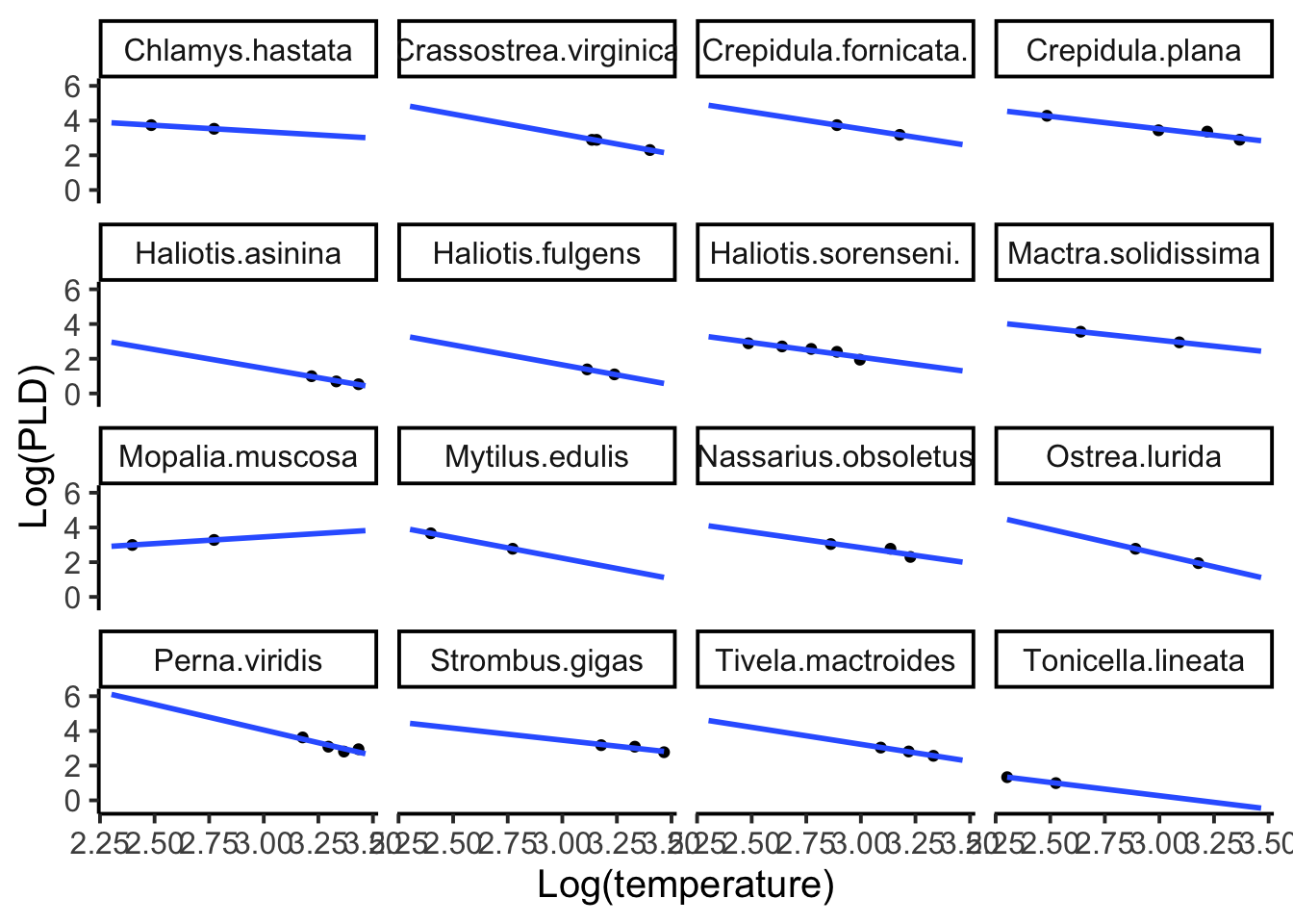
We will use the lme4 library and the well-known lmer() function for our linear regression models with random effects.
library(lme4)

# Mixed model with random effect for intercept
mix.int <- lmer(l.pld ~ l.temp + (1 | species), data = mol)
summary(mix.int)
## Linear mixed model fit by REML ['lmerMod']
## Formula: l.pld ~ l.temp + (1 | species)
## Data: mol
##
## REML criterion at convergence: 43.7
##
## Scaled residuals:
## Min 1Q Median 3Q Max
## -2.37222 -0.32686 -0.09382 0.43821 2.34871
##
## Random effects:
## Groups Name Variance Std.Dev.
## species (Intercept) 0.86457 0.9298
## Residual 0.03309 0.1819
## Number of obs: 44, groups: species, 16
##
## Fixed effects:
## Estimate Std. Error t value
## (Intercept) 7.1728 0.5284 13.575
## l.temp -1.5175 0.1592 -9.531
##
## Correlation of Fixed Effects:
## (Intr)
## l.temp -0.896The above model summary looks somewhat similar to the output from an lm() model object. Skipping down to the Fixed effects section, those are the estimates for the fixed slope, and the grand mean of the intercept. Note that the effects summary ends with the test statistic (t value) and no p-values are reported. The reasons for that are lengthy, but can be read about here (cite). Although the intercept is listed under Fixed effects, the intercept really was a random effect, and can be see in the above section, Random effects. The Name column tells us the parameter is the intercept, and the factor is listed under the Groups column, indicating we have a random intercept for each species. We then get a variance and standard deviation for the random effect (along with the residual). So where are all these species-specific intercepts we have been promised? Individual factor level random effects are not part of the summary, and for many models the number of factor levels would make the summary output very long. But the species-specific intercept coefficients can be easily found with the coef() function.
coef(mix.int)$species## (Intercept) l.temp
## Chlamys.hastata 7.612748 -1.51751
## Crassostrea.virginica 7.592515 -1.51751
## Crepidula.fornicata. 8.045609 -1.51751
## Crepidula.plana 8.063220 -1.51751
## Haliotis.asinina 5.807247 -1.51751
## Haliotis.fulgens 6.083069 -1.51751
## Haliotis.sorenseni. 6.688210 -1.51751
## Mactra.solidissima 7.589660 -1.51751
## Mopalia.muscosa 7.061086 -1.51751
## Mytilus.edulis 7.141801 -1.51751
## Nassarius.obsoletus 7.370159 -1.51751
## Ostrea.lurida 6.967626 -1.51751
## Perna.viridis 8.144314 -1.51751
## Strombus.gigas 8.048942 -1.51751
## Tivela.mactroides 7.677603 -1.51751
## Tonicella.lineata 4.871674 -1.51751It’s clear that each species has it’s own intercept, yet all the slope coefficients (l.temp) are the same (fixed).
9.6.1.2 Interclass Correlation Coefficient (ICC)
A mixed model with a random intercept is also a point where we can pause and run a diagnostic called the Interclass Correlation Coefficient (ICC), which is a sort of indicator for how much group-specific information is available for a random effect to help with. An ICC functions similarly to an ANOVA in a sense that it looks at the variability within groups compared to the variability between groups. In the below ICC figure you can see how the group with low ICC has observations within groups that don’t necessarily cluster.
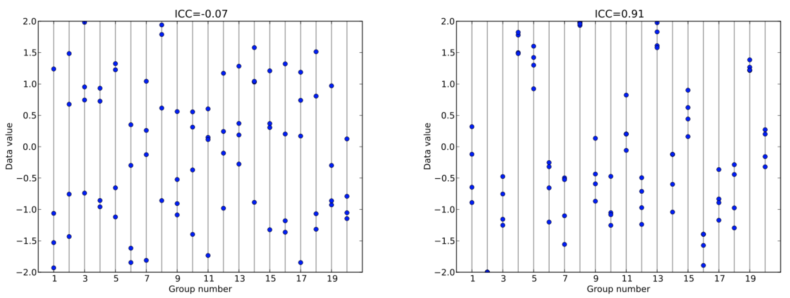
Figure 9.2: Example ICCs estimates and how the group level information contributing to that ICC may look.
In fact, if I were to give you a value of 0.5 you would have a very hard time guessing as to which group that observation would likely belong to. Conversely the ICC of 0.91 is a very high ICC and suggests that there is a lot of group specific information within the data. Again, if I gave you a specific data value such as 1.0 you would be quite confident in understanding which of a small number of groups that value would likely to be contained—and which groups it would not be in. It is worth noting that ICCs range from 0 to 1, much like a correlation coefficient and that ICCs closer to 0 are considered to have low group level information while ICCs approaching one are considered to have higher amounts of group level information. The cutoffs for weak, moderate, and strong ICCs are subjective and subject to debate (cite). The formula for ICC is also fairly straightforward in which we are just looking at the proportion of the random intercept variance compared to the total variance within the model.
\[ ICC = \frac{\sigma_{\alpha}^2}{\sigma^2+\sigma_{\alpha}^2} \] In our mixed model with a random intercept, \(\sigma_{\alpha}^2 = 0.86457\) and \(\sigma^2 = 0.03309\). Do the math, and we get an ICC of 0.96, which is a very high ICC and strongly suggestive that there is within-group variability that would benefit from a random effect.
9.6.1.3 Fixed intercept, random slope model
Maybe we want to entertain a random slope, because we hypothesize that the effect of our predictor differs among groups. And maybe we want to fix the intercept because we know that all groups start in a similar place. For example, consider an organism growth study were a random effect for slope is needed to capture the different growth rates, but a fixed intercept may be useful because all organisms start at the same size. Let’s try this mixed effects model with the mollusc PLD data.
# Mixed model with random effect for slope
mix.sl <- lmer(l.pld ~ l.temp + ( 0 + l.temp | species), data = mol)
summary(mix.sl)
## Linear mixed model fit by REML ['lmerMod']
## Formula: l.pld ~ l.temp + (0 + l.temp | species)
## Data: mol
##
## REML criterion at convergence: 47.8
##
## Scaled residuals:
## Min 1Q Median 3Q Max
## -2.54025 -0.41731 -0.03549 0.50757 2.18100
##
## Random effects:
## Groups Name Variance Std.Dev.
## species l.temp 0.11241 0.3353
## Residual 0.03581 0.1892
## Number of obs: 44, groups: species, 16
##
## Fixed effects:
## Estimate Std. Error t value
## (Intercept) 7.3323 0.4842 15.144
## l.temp -1.5838 0.1843 -8.594
##
## Correlation of Fixed Effects:
## (Intr)
## l.temp -0.889Again, we can see our fixed effect for the intercept and the global mean for slope (l.temp). The variance in our group-specific slopes for species is 0.11, but we are much more likely to be interested in the actual slope coefficients.
coef(mix.sl)$species## (Intercept) l.temp
## Chlamys.hastata 7.332336 -1.409631
## Crassostrea.virginica 7.332336 -1.438006
## Crepidula.fornicata. 7.332336 -1.283611
## Crepidula.plana 7.332336 -1.277271
## Haliotis.asinina 7.332336 -1.977311
## Haliotis.fulgens 7.332336 -1.912372
## Haliotis.sorenseni. 7.332336 -1.750873
## Mactra.solidissima 7.332336 -1.427474
## Mopalia.muscosa 7.332336 -1.610111
## Mytilus.edulis 7.332336 -1.595278
## Nassarius.obsoletus 7.332336 -1.506000
## Ostrea.lurida 7.332336 -1.640789
## Perna.viridis 7.332336 -1.273649
## Strombus.gigas 7.332336 -1.301470
## Tivela.mactroides 7.332336 -1.410386
## Tonicella.lineata 7.332336 -2.527107Slopes certainly do vary all the way from -1.3 to -2.5, while our intercepts are the same as we expect.
If you are looking closely at the estimates between the models, you might notice something. The global mean estimate for the random intercept, fixed slope model was 7.17, while the fixed effect estimate for the intercept in the random slope, fixed intercept model is 7.33. This is not a huge difference, but it is noticable and brings up the question why would these estimates differ? One is a pure fixed effect and the other is the mean of the random effects, but we might expect them to be similar? What is going on is that both fixed and random effect estimates are subject to change depending on what else is in the model. This is functionally no different than predictor coefficients changing as you add predictors to a multiple linear regression. But with fixed and random effects, these changes can be a result of the constraints that are imposed or removed on parameters. These coefficient differences are rarely anything to be aware of or concern with, but it is worth knowing that coefficient estimates from one mixed model are not insured when changing the model, even if the data stay the same.
9.6.1.4 Random effects model
Perhaps you are now thinking that either the fixed intercept or the fixed slope are too constraining. This is often the case, and the good news is that a random effects model—a model with both a random intercept and random slope—is often a good choice. A random effects model allows the flexibility for each group to have it’s own unique regression relationship, only informed by the grand means if lacking information on their own. And as discussed earler, the constraints experienced by the random effects when another effect is fixed, are all but gone.
# Random effects model (both intercept and slope are random)
re.mod <- lmer(l.pld ~ l.temp + (l.temp | species), data = mol)
summary(re.mod)
## Linear mixed model fit by REML ['lmerMod']
## Formula: l.pld ~ l.temp + (l.temp | species)
## Data: mol
##
## REML criterion at convergence: 41.4
##
## Scaled residuals:
## Min 1Q Median 3Q Max
## -1.45479 -0.43418 -0.00315 0.38145 1.55807
##
## Random effects:
## Groups Name Variance Std.Dev. Corr
## species (Intercept) 5.04311 2.2457
## l.temp 0.48021 0.6930 -0.91
## Residual 0.01854 0.1362
## Number of obs: 44, groups: species, 16
##
## Fixed effects:
## Estimate Std. Error t value
## (Intercept) 7.5719 0.7257 10.43
## l.temp -1.6253 0.2305 -7.05
##
## Correlation of Fixed Effects:
## (Intr)
## l.temp -0.946Let’s skip directly to the coefficients.
coef(re.mod)$species## (Intercept) l.temp
## Chlamys.hastata 6.796156 -1.2055908
## Crassostrea.virginica 8.978195 -1.9457251
## Crepidula.fornicata. 8.828618 -1.7730084
## Crepidula.plana 7.912251 -1.4661045
## Haliotis.asinina 7.384957 -1.9939835
## Haliotis.fulgens 7.141784 -1.8536288
## Haliotis.sorenseni. 7.096306 -1.6659621
## Mactra.solidissima 7.347379 -1.4314843
## Mopalia.muscosa 3.393358 -0.1009882
## Mytilus.edulis 8.617624 -2.0872607
## Nassarius.obsoletus 8.032936 -1.7325796
## Ostrea.lurida 9.267637 -2.2760165
## Perna.viridis 10.208954 -2.1386522
## Strombus.gigas 7.746908 -1.4249938
## Tivela.mactroides 8.365923 -1.7307560
## Tonicella.lineata 4.031327 -1.1776601We can see that both random intercepts and random slopes vary a lot—much more than in the mixed effects models. This does not mean the random effects model is better, as some of this variability could be coming from noise, but overall, we can safely assume that both model parameters are free to explore a wider parameter space for each group and likely estimating group-specific relationships that are as accurate as we can get.
So how do all these estimates compare with each other? Below, we will compare the extremes. A disaggregated model (one common model for every species), a species-specific model (each species is fit using only data from that species), and our random effects model.
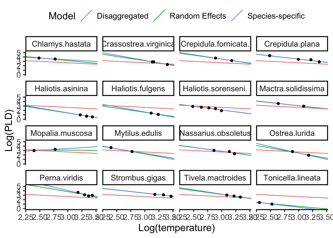
It is clear that the disaggregated model is not a good model. We know species need to be accounted for, and yet the disaggregated model fits several species very poorly. The species-specific model fits and the random effects model fits are often closely estimated, suggesting that one might not be significantly superior over the other. And while that may be true to some extent, we now know that random effects model is providing several behind the scenes benefits. Poorly estimated groups are informed by the grand mean parameteres, and we are running the whole analysis in one model. Perhaps most importantly, we know that species in this case, is a classic random effect, and just having that random effect in our model increases the realism between our model and the system we are seeking to describe.
9.7 Should I Consider Random Effects?
When considering a random effect, it can be informative to ask the following quesitons.
- Can the factor(s) be viewed as a random sample from a probability distribution?
- Does the intended scope of inference extend beyond the levels of a factor included in the current analysis to the entire population of a factor?
- Are the coefficients of a given factor going to be modeled?
- Is there a lack of statistical independence due to multiple observations from the same level within a factor over space and/or time?
Now let’s answer those questions with the PLD data.
Answers with the PLD data 1. Can the factor(s) be viewed as a random sample from a probability distribution? Both the individual species used for the analysis and the relationship between temperature and PLD could be viewed as a random sample from a probability distribution. Species can be viewed as a random sample of all species, and the relationship (slope) between temperature and PLD for each species can be viewed as being drawn from a distribution of slopes.
Answer: Yes
2. Does the intended scope of inference extend beyond the levels of a factor included in the current analysis to the entire population of a factor? O’Connor et al. (2007) were interested in examining the generality of the temperature-PLD relationship, and therefore the scope of inference was not restricted to the 72 species analyzed, but rather to all marine animals with a planktonic larval stage.
Answer: Yes
3. Are the coefficients of a given factor going to be modeled? If there is variation among species in average PLD, then ask “why might species differ in their average PLD?” It is hypothesized that this might be due to evolutionary processes driven by regional temperature variability. To test this hypothesis, you could add species-level predictor variables to the model.
Answer: Could be
4. Is there a lack of statistical independence due to multiple observations from the same level within a factor over space and/or time? For the O’Connor et al. (2007) analysis, multiple observations existed for each of the 72 species.
Answer: Yes