Chapter 5 Models and Estimation
5.1 Introduction
One of the most critical concepts in basic statistics is to be aware of the fact that a statistical model and a statistical estimation procedure are two different things that both go into your analysis, and often times can both be manipulated. Too often in introductory statistics training, the focus is on the model—and the estimation is along for the ride. Even if you adopt a single estimation procedure and stick with it, it remains important to learn from the start that you have options. For example, simply because you want to use an ANOVA model does not mean you are required to use a Frequentist estimation procedure. A model and an estimation procedure are like a car and driver—you need both to get where you are going, but changes to either could result in the experience of how you get where you are going or where you end up.
Models are the machinery—the car in the previous example—which can be thought of as a description of the system, process, or relationship you are trying to evaluate. The hardware of the model is the parameters, which can be as simple as a single parameter for modeling the mean of something, to much more heterogeneous collections of variously-related terms that seek to explain complex systems. The estimation is what makes the model work, or the context in which the parameters are estimated. Estimation has philosophical underpinnings because it provides inference to how we interpret the data and system. So although you could have the same model and same data used twice, a different estimation procedure could lead to different results or inferences (but it is worth saying that often the philosophical interpretation is a greater difference than the results). We can end here with the car metaphor, but it would be worth mentioning that data would be the fuel for the car.
5.2 Models
Model is perhaps the most used term in a statistical context, and its continued reference and importance are warranted because the model you are using represents your idea of the system, process, or relationship you are seeking to describe. (Although system, process, and relationship are all appropriate ways to think about a model, I will generally adopt the term system.) If you have an accurate model for your system, then you will have a better idea of the quality of your data, the inference of your parameters, and generally get much farther in your analysis. If your model is flawed to the point of not being accurate enough to be useful, then your analysis will at best be incorrect but runs the risk of being misleading. When we think about incorrect models in ecology, sometimes the stakes are not that high, but consider a misleading model for a cancer drug treatment, or some other application where human lives are involved. We all want to use a good model, but we must also realize that models are only representations of (often complex) systems, and cannot be perfect. It’s overstated in statistical ecology, but still correct, that ``All models are wrong, but some are useful.’’ (–George Box?)
When talking about a statistical model, it’s important to first distinguish it from a mathematical model. A simple way to remember the difference between a mathematical model and statistical model is that a mathematical model does not contain a term (parameter) for error. When a mathematical model is expressed, we can solve for a term and know what that term is or what it could be (if more than one possible answer exists). For example, \(5 = 2 + x\) would suggest that \(x = 3\). However, a statistical model includes a term for error because we are describing a system that is not perfectly known and for which some uncertainty exists. A useful way to conceptualize a statistical model is to think about the left side of the equation as the response and the right side of the equation as the combination of the deterministic part of the system plus the stochastic part of the system. The deterministic part of the system is the model, or the relationship you are seeking to test or confirm. The stochastic part of the system is the random error or deviations from the relationship that are unexplained by the model. Chapter 5 (Linear Models) goes into more detail on the mechanics of these model elements, but let’s continue with an example just to apply the model concept to something.
A simple description of a statistical model:
response = deterministic + stochastic
Consider a very simple model in which your data include observed rainfall and plant growth (for some number of individual plants in a growing season). The response variable (\(y\)) would be plant growth (e.g., size) and the data we think determines the response (\(x\)) is precipitation. The system we seek to describe here is that precipitation effects plant growth, and we could extend this to hypothesize that increases in precipitation result in increases in plant growth—so we are not just saying that there is a relationship, but we are guessing as to the direction of that relationship. This might be a very defensible model—who would challenge that precipitation does not positively effect plant growth? Although there is a good chance that this is a useful and realistic model, it is also reasonable to think that other factors go into determining plant growth. For example, what about sunlight, nutrients, and temperature, just to name a few possible growth factors. The reality of the system is that a long list of variables likely go into determining plant growth, and that there are variables we don’t even know about or cannot measure. This uncertainty in the system is what results in random error—or the stochastic part of the model that captures the deviations from the expected relationship. It is perfectly reasonable and expected to have random error in a statistical model, but it is also appropriate to think about how that error is generated, what it looks like, and how we can minimize it while still acknowledging it. A deeper look at model error can be found in Chapter 5.
Once we have acknowledged that there will be error in our model, we focus on the deterministic part of the model. The deterministic part is simply how we perceive the system or relationship to work. In a simple linear regression model, we would expect that the increase in \(x\) results in some change in \(y\), and that this change is constant across all values of \(x\). (If the change is not constant, we can still find a model for that, but it might not be simple linear regression.) The description of the model takes place using terms called parameters and mathematical operators (e.g., addition and subtraction). Parameters are unobservable, but we can still estimate them and their effects by using the data we have. Going back to the plant growth example, we might find that an increase in precipitation results in a very small increase in plant growth, which would estimate a parameter—expressed as a coefficient—that is a small positive number. Or, we might observe very large increases in plant growth with increasing precipitation, which would result in a parameter coefficient that is a large positive number. In both of these cases we have not directly observed the parameter at all, but we have used the data to estimate and better understand the parameter based on available information. It is also possible that we might see no effect of precipitation on plant growth. In this were observed there are many possible explainations: we did not have enough of a range of preciptation values to detect a difference, other factors (e.g., sunlight, etc.) are equally or more important and need to be considered, we were studying plant species that store water and thus don’t readily respond to short-term precipitation, and so on.
5.3 Model Complexity
It is clear that there is a wide range of how useful models can be. The goal of just about all modeling work is to find, develop, or otherwise implement a model that balances generalizability with complexity. We want a model to be general enough that it contains truths and can be applied elsewhere, but not so general that it does not advance our understanding of the system. Similarly, we want enough model complexity such that our model is not overrun with error or too simplistic, but we also want to avoid using a model that is to complex that it becomes a product of its own data and is not useful for any other purposes. You may hear models that are too general referred to as underparameterized, and models that are too complex as overparameterized. For instance, if we agree that exercise is good for living longer that may be true, but is a very generalized model. How much exercise is good and how much longer would a person live with one more unit of exercise? The pure relationship between exercise and longevity is simply not very operational because other relevant factors go into this system. In this case, the model is too generalized to be useful. On the other extreme, if we decided that exercise, plus diet, plus genetics, plus 20 other factors went into longevity, we might end up with a better fitting model, but not necessarily a better overall model. Our overfit longevity model might be unrealistic for most poeple who do not have all the data required to estimate longevity, in addition to the other risk that the parameter coefficients could be too sensitive to the data used to fit them, and if the health dataset we used did not have a representative sample of all people, it could produce biased estimates for those using the model. Realistically, a model for longevity might be optimized by including exercise, diet, and family history. That’s not to say that these are the only relavent longevity predictors, but they might be the most important and also make the model available to the maximum amount of people.
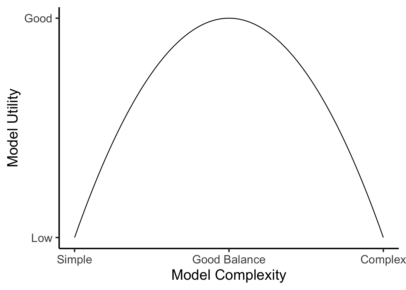
Figure 5.1: General relationship between model complexity and model utility, whereby the highest model utility is typically achieved for models that are not too simple and not too complex.
Model selection is a term you hear frequently used in statistics. Model selection has become very popular over the last few decades largely due to new techniques and software that are able to explore a large number of models. But it remains important to consider what the goal of model selection is. Is your goal prediction, for example predicting unobserved information? Or is your goal understanding, as in understanding relationships within the data you’ve already collected? It remains important to remember that model selection occurs on the front end, too, and may not be an explicit test you run on the data, but simply exercising discretion in which terms you decide to include in the first place.
5.4 Estimation
As we covered earlier, the model is kind of like the car, with the engine being the parameters. But a car and engine alone doesn’t necessarily get you where you need to go. Estimation is how we use our model, or how we allow the parameters to be figured out. A number of different estimation types exist within statistics; however, will cover three common estimation types here.
The first estimation type is perhaps the least frequently used and is called Monte Carlo estimation, or sometimes bootstrapping or resampling. This is an estimation type which requires very few assumptions and uses the observed data over and over to draw inferences.
The second type of estimation is the most common and is referred to as frequentist estimation or Fisherian estimation (after R.A. Fisher). Frequentist estimation assumes a parametric distribution and is interested in the long run of frequencies within the data. Most statistical software that don’t specify otherwise default to using some type of frequentist estimation—typically least squares or maximum likelihood.
The third and final type of estimation that will cover here is called Bayesian estimation. Bayesian estimation is actually centuries old but has been revitalized in the past few decades because of the computational complexity that is required to estimate in a Bayesian framework. Bayesian inference is also assume a parametric distribution. Bayesian estimation includes a prior distribution or prior knowledge about the parameter.
Regardless of the estimation type you use perhaps the most important recommendation is to report your estimation type in sufficient detail and assume that no one is making assumptions about how you’ve estimated the parameters in your model.
5.4.1 Monte Carlo Estimation
Let’s look at Monte Carlo estimation in an example. Consider a null hypothesis which is defined as the pattern in the data being no different from what is occurring in nature. After we collect data, we develop a test statistic, and then randomize the data and generate a large number of test statistics from the randomized data. All of the randomized test statistics create a null distribution, which we then used to compare to our observed test statistic.
Consider the data set below which is a fictitious data set about phytoplankton density inside and outside a Mississippi River plume.
| Inside Plume | Outside Plume |
|---|---|
| 12 | 9 |
| 15 | 7 |
| 21 | 9 |
| 22 | 14 |
| 15 | 8 |
| 17 | 13 |
Inside the plume we have six values with a mean of 17 and outside the plume we have another six values with a mean of 10. Here our null hypothesis would be that there is no difference between phytoplankton densities inside or outside the plume. We’ve also calculated the mean difference, or average difference between our groups, which is 7 and we might call \(D_{Obs}\). In order to run the estimation we need to run a number of simulations. The number of simulations may range from hundreds to millions and largely depends on the complexity of the data and the computational power available. However, for each simulation the approach is the same. Each simulation randomly assigns all 12 observations in the data to one of two groups. This random assignment between groups is meant to simulate the null hypothesis that any of the observations could be coming from either group because there are no differences between groups. For each simulation a difference between the two groups is calculated and we might call that difference \(D_{Sim}\). From the large number of simulations we have a large number of \(D_{Sim}\)s and we can use these \(D_{Sim}\)s to create what is called a null distribution. We then compare our \(D_{Obs}\) value, which was 7, to the null distribution and use probability to interpret whether the \(D_{Obs}\) value falls within a high or low probability region of our null distribution. In other words, is the observed difference the same all the other differences we could simulate, or does it really stand out? Often because of their simplicity Monte Carlo methods and bootstrapping methods are again the least common of what we use in the natural sciences; however, the underlying concepts of how they work remain important.
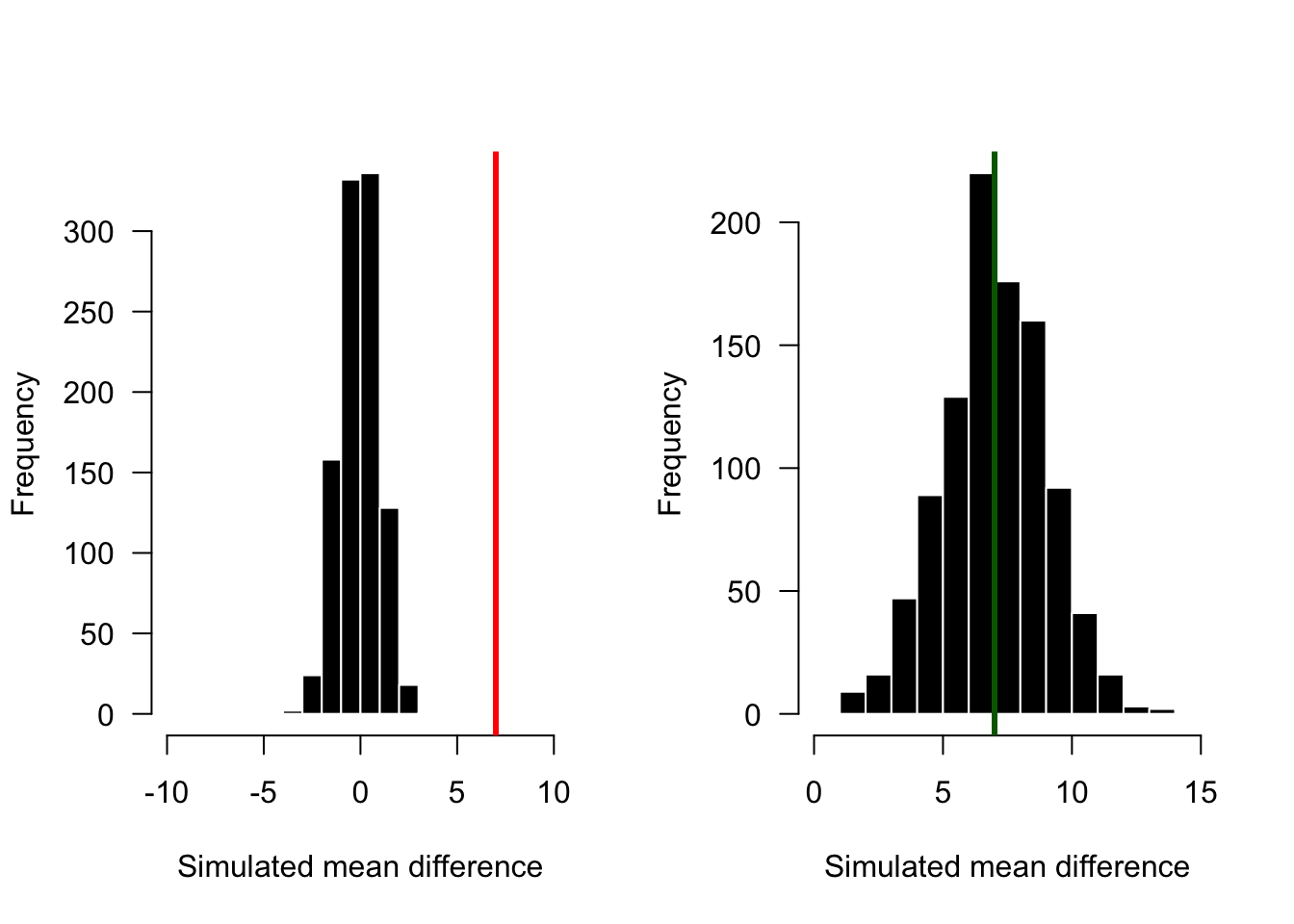
Figure 5.2: Two hypothetical outcomes from a simple Monte Carlo test. If the observed difference is 7, this observation would be significantly different from the null distribution in the left panel, where 7 (the red line) falls far outide the null distribution. However, in the right panel, 7 falls in the middle of the null distribution, suggested that the observed difference is no different than the randomized differences.
5.4.2 Frequentist vs Bayesian
Next let’s consider both frequentist and Bayesian estimation at the same time. We will do this not only because these are the two most common types of estimation that you will encounter, but also because their differences in many ways contrast with each other and a direct comparison can be useful. Frequentist approaches can be thought of as asking “What is the probability of the data that I observed compared to a fixed and unknowable parameter(s).” Bayesian estimation provides the opposite interpretation, asking “What is the probability of certain parameter values based on the data I observed.” Although these statements may seem similar, they are in fact incredibly different.
The frequentist paradigm:
- Assume that data are repeatable random variables.
- Assume that parameters do not change and are often referred to as fixed and unknowable.
- All experiments are considered to be independent in the sense that no prior knowledge can be (directly) provided to a parameter estimate or model.
- Frequentist this outcomes are driven by point estimates and ultimately is null hypothesis driven in the sense that we accept or reject hypotheses and outcomes.
- p-values are a key outcomein frequentist estimation.
In contrast, Bayesian approaches are quite different. Bayesians:
- Assume that the data are fixed; in other words, the data are the things that are knowable and parameters are random variables that we are seeking to estimate (based on the known data).
- Adopt a degree-of-belief from probability.
- Can update beliefs in the sense that prior information can be used to directly inform the estimate of certain parameters.
- Bayesian estimation is driven by distributions and uncertainty (as opposed to point estimates). 5. Outcomes are not required to accept or reject anything based on a critical value; instead probabilistic interpretations of outcomes are generated that may not distill to a simple yes or no but may in fact be more realistic to the question at hand.
Put another way the frequentist asks “The world is fixed and unchanging; therefore, given a certain parameter value how likely am I to observe the data that supports that parameter value?”
While the Bayesian asks “The only thing I can know about the changing world is what I observe; therefore, based on my data what are the most likely parameter values I could infer.”
5.4.3 Why the frequentist popularity?
You may not have switched your philosophy to a Bayesian approach at this point, but you may also be seeing the intellectual attractiveness in it. So the question becomes why have frequentist approaches dominated and why might this be the first time you are hearing about Bayesian estimation? Frequentist approaches were popular for much of the 20th century and this is largely due to a number of reasons. Frequentist approaches are often operationalized within simple point and click routines and they do not require much computational power. As you may learn Bayesian approaches can often require a lot of computational power making them challenging to implement (until the advent of modern computers). Another factor is that frequentist approaches or largely developed by R.A. Fisher who also popularized the analysis of variance or ANOVA. Although ANOVA is a model that can be estimated using different estimation techniques it does help your cause when an incredibly useful model is developed in parallel to an estimation routine. Finally p-values have also helped the popularity of frequentist approaches. Although you may have questioned p-values yourself or read articles about concerns with using p-values, the reality for many people is that an accept reject framework remains simplistically attractive for interpreting outcomes.
5.4.4 The problem with p-values
As convenient as p-values may be there are a number of problems with them. These problems are increasingly being cited and reported, and whether you use p-values or not you should be aware of them. First off p-values are oftentimes not intuitive and can be hard to explain. Second, a p-value does not indicate whether a result is correct or not, nor does it provide information about the magnitude of an effect. p-values really just provide a binary interpretation of something, yet in many instances we don’t want a binary interpretation or we make inferences on the p-values number that are not accurate to be made.
5.4.5 What we can agree on
So what can we agree on when it comes to estimation? It may be fair to say we can agree that we all want our models to fit our data as well as can be which is often measured by the residuals. Choosing your estimation may end up being a philosophical exercise for those interested in the deeper aspects of estimation, or it may be a technical exercise for those that favor certain statistical approaches that may be grounded in one estimation.
5.5 The Mechanics of Estimation
5.5.1 Maximum Likelihood
For frequentist estimation we often use maximum likelihood estimation, or MLE. MLE maximizes the log function by minimizing the negative log likelihood. R does this for you but you’re encouraged to know how it is done and the numerous variants of MLE that may be used in different models. For instance least squares estimation is simply minimizing the sum of squared errors and is a simpler version of MLE. And if a linear model has normal errors, we call MLE OLS, or ordinary least squares.
5.5.2 Bayesian Estimation
Bayesian estimation requires a bit more in terms of the mechanics. The basis for Bayesian inference is Bayes rule which includes a term for the posterior distribution the likelihood function the prior distribution and a normalizing constant.
\[ p(\theta|y)=\frac{p(y|\theta)p(\theta)}{p(y)} \] or
\[ Posterior = \frac{Likelihood \times Prior}{Normalizing Constant} \]
The posterior distribution is really just another way of saying the result. The posterior distribution is the outcome of our estimation, but because it is in the form of a distribution and not a point estimate we call it a distribution. The likelihood function can be a number of different likelihood functions but is often very similar to maximum likelihood and this is a shared feature with frequentist estimation. The prior distribution is the ability to add existing parameter information to a model. For instance you may know that a parameter estimate needs to fall within a certain range of values. The priority distribution is one option you have to implement that prior information before the model begins to estimate the parameters. Finally the normalizing constant is something that, to simplify, allows the results of the estimation to be interpreted in a probabilistic framework.
So how does all this work?
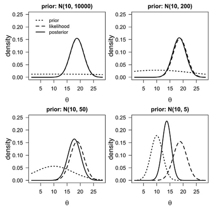
Figure 5.3: Example of priors of different strength, and how the influence the posterior distribution. (Source: XXX)
In this figure you can see how prior information may or may not inform your parameter estimate (posterior distribution). In the upper left hand corner you see how a prior distribution (dotted line) is flat and is basically contributing no information to the posterior (solid line). In this case the likelihood, which is the dashed line that you can barely see, is nearly identical to the posterior, which is the model output. Again in this case the data within the model are almost exclusively informing the outcome, as you might expect. In the other three panels you see the prior gradually increase in the amount of specific information it provides. As it does that you can see the posterior distribution take on some of that information between the prior distribution and the likelihood. In fact, by the bottom right hand corner (the panel with the strongest prior) you see that the posterior is really a combination estimate of that which is provided by the prior and that which is provided by the data (or likelihood).
5.6 Final Advice
Ultimately, you’re encouraged to learn more and understand the estimation that you use. Unfortunately estimation is often assumed leaving the reader unable to know exactly what was done or how to replicate it. Always consider that models and estimation are separate components of your analysis and in the vast majority of cases each can be specified, meaning a certain model can be estimated in different ways or different estimation procedures can be applied to the same model.