Chapter 2 Learning R

2.1 Introduction

R is the programming language that will be used to implement and explore the analytical and statistical concepts presented in this book. The term language is an appropriate one because R is not necessarily inventing any new statistical tests or making large conceptual contributions to analyses (although that comment can be debated later). Rather, R is simply the set of terms, expressions, and syntaxes we use to implement the analyses we want. It’s a bit of a forced comparison, but if we were studying the Renaissance (as opposed to data analysis), we might want to learn the language of Italian, so that we can best understand and interpret the material, the same way that we might want to learn R if we want to think analytically and statistically about data and systems. (Disclaimer: you can certainly study the Renaissance without knowing Italian, and you can also conduct data analysis without knowing R.)

This chapter is designed to get you comfortable using basic operations in R. This chapter is not designed to be a comprehensive and lengthy instruction manual on R. First off, there is a large number of excellent resources available to thoroughly teach you R, if that is your primary objective—so there is no reason to reinvent the wheel. In fact, please see the end of this chapter for a list of recommended resources. Second, in many cases there are so many ways to do the same thing in R, that it can become restrictive to try to specify one approach. And as such, being comprehensive about R can result in being overwhelming. Finally—and perhaps most importantly—this text is focused on exploring data analytic approaches and statistical concepts first, and learning R second. However, to be more accurate, this text takes a hybrid approach of teaching R jointly with data analyses, partly because any instruction on applied analyses requires some language or program to carry out functions (so why not R?).

Additionally, as a side-effect, there can be cognitive value in learning how R perceives information. For example, learning R may mean that you no longer think about your data as a spreadsheet, but more accurately as vectors, or data frames, or matrices. Because so many things in R can be both broken down to their elemental level or contribute to a larger object, there can often be analytical clarity when the study system is also deconstructed.

So if this chapter is not designed to teach you everything you need to learn to command R, then what is the objective? The objective is simply to expose you to R and to get you comfortable with it. Even after many years of coding, it can be inefficient to try and learn something in R by memorizing it. But it can be effective to know basic functions and structures, and then how to find reliable help when you come up against new material. For those readers who have never used R, it may seem daunting at first. Partly, this is an accurate impression as R is hugely powerful and complex, so we should all be humbled by what it can do. However, you will find that (in general) using R is so deconstructable that you can also pick apart things to see how they work. Syntaxes and terms are generally consistent and functions are readily broken into their component arguments. For those readers who have experience in R, let this chapter serve as a refresher of basic operations that are foundations for data manipulation and analysis.

The introductory material on R is organized into three sections. The first section, Up and Running, is the absolute basics of how to get R, what R is, and how to take the first steps in a programming language. The second section, Data Uploading and Manipulation, concerns how to work with a dataset in R and what basic and useful manipulations are. Finally, there is a small section on Plotting. Although plotting be covered in greater depth in later chapter, there is tremendous value in being able to quickly visualize (raw) data, and as such, the information here is more of a first-aid kit for plots—Chapters 10 and 11 are where you can read about major surgery for visuals.

2.2 Up and Running

So what is R? R is a command-line programming language that is not a statistical software per se, but certainly has statistical applications. R was first written in 1993 by Ross Ihaka and Robert Gentleman at the University of Auckland, New Zealand, and was built off the S programming language. There have been many updates and developments in R since it was first introduced, and it is now widely used by statisticians and those in similar fields.

What is command-line programming? Command-line programming means that the user enters strings of text into a command-line interface that are then read and executed by a program. It is a simple way of using a computing language to precisely tell a computer or program exactly what you want it to do, and doing so without dropdown menus, buttons, and other graphical features. If that doesn’t make sense and/or you are a millenial, just picture a computer from the 1980s where you had to type everything into the computer that you wanted it to do—that is command-line programming. Command-line program can be wonderfuly freeing and simple in it’s simplicity—the program only does what you tell it to do. But for those who are used to clicking a mouse and other graphical interfaces, command-line programs can be tedious and hard. Fortunately, R has options for integrated development enviroments (IDEs), including R Studio. R Studio is an IDE that integrates the command-line experience of R with other orgnanizational components, such as panels to view plots, quick access to help files, and a script editor, which will be discussed below.

How popular is R? R is incredibly popular. Despite the fact that R is popular, it can be hard to come up with a singular objective piece of evidence demonstrating R’s popularity. This is because R has a wide user base that spans disciplines from academics to healthcare to industry. The metric of using R is also hard to pin down—should this be number of times people have downloaded R, which is a very liberal interpretation of using R? Or should it be citations in published literature, which is a very conservative interpretation of using R? Also, comparing the popularity of R is really only effective if we know the popularity of other software, and quantifying all of these software usage statistics is challenging and uncertain. Rather than focus on how we cannot demonstrate the numerical popularity of R, we can list the ways in which R demonstrates popularity. For example, R has spawned a number of communities, which are simply networks of R users that interact around some aspect of R. R also has an annual conference that has been going on for almost two decades at locations across the globe. There is also an R journal (The R journal), which is entirely dedicated to the development of R. Finally, as of this writing, R has 17,022 contributed packages. We will talk more later about what exactly a package is, but the point here is that packages are user-driven contributions that can be made to work with R, and the broad support and use if R has clearly led to a very large number of packages.

How current is R? R is very current and stays current through version updates that happen a few times each year. R studio, a popular R integrated development environment (IDE) that works hand-in-hand with R is also updated frequently. And as mentioned in the above paragraph, the R user base constantly contributes and updates packages, which means that not only is R current, but it is constantly growing.

How do I get R? R is free and downloading it is very simple. If you visit www.r-project.org, there are directions to download. (Briefly, you will be directed to a CRAN Mirror and it is advised to select the location nearest to you. CRAN stands for the Comprehensive R Archive Network, and a mirror is just a duplicate place from which R can be downloaded in order to reduce the demand on one location.) Obviously you need to download the version of R that matches your operating system, and the rest of the download and install should proceed like any other software.

It is advisable to also download R Studio. As mentioned above, R Studio is an integrated development environment (IDE). R Studio is not the only IDE available for R, but it is by far the most popular and very user friendly. R Studio basically provides a dashboard for your R experience. If you download and run just R, you will get a minimal experience—a console for compiling code—and you will need to open other files if you want to use a script, view plots, etc. R Studio has identified the most popular functionalites of R—like having a dedicated script, plotting window, package library, instant help files, etc.—and integrated them into one application. R Studio still directly works with R, but it just makes the experience much smoother. One analogy comparing R to R Studio is that R is like a text editor software while R Studio is like Microsoft Word. Both can handle text, save it, print it, and do other basic functions, but Microsoft Word provides an integrated environment where document structure, formatting, images, and other functions can be easily included. R Studio can be downloaded and installed for free, from www.rstudio.com. (Note that there are pay versions of R Studio, but if you are in need of that amount of product and support, you probably should be reading another book.)

Console vs Script? R Studio will open to four windows (that are manipulable and customizable). One window will show you your environment, which includes primarily the objects (data, models, etc) that you have run and saved and can be recalled. Another window will include a directory for the files in your working directory, a tab for showing plots, a tab for package management, and a tab for help files. The other two windows consist of the R console and a script (though technically if you open R Studio a script may not be open and you will need to go to File > New File > R Script to get a script).

You can tell the console because it opens with the R version information and disclaimer:

R version 4.0.3 (2020-10-10) -- "Bunny-Wunnies Freak Out"
Copyright (C) 2020 The R Foundation for Statistical Computing

This console is where you put things that you want to run in R. Commands and functions in console will be on lines starting with

and when you hit return, the console will compile your code. This is a good thing! But it is not a great place to put code that is in development. A script (basically a text file with the file extension .R) is the place where you will want to put code that you are developing and don’t want to continually run. Think of it this way: the console is like a typewriter—what you put in, you will get out, but once you put it in, it’s not efficient to try and go back. In contrast, a script is like a word processing document—you can type, delete, and format until your heart is content, and none of it becomes official until you print that document. In fact, one the main benefits of scripts is that you can add comments, which are simply pieces of text that follow the #, which means that they are not compiled by R. Comments are incredibly useful to make notes or document things you do in your code.

It is extremely recommended that you code in a script, which is not only a small file size, robust to corruption, and good for collaboration, but also very easy to run. In R Studio, you simply need to highlight code you want to run, and with a keystroke it will be delivered to the console for processing.

Packages and Libraries R has become very package-intense, which comes with challenges, but overall has been a tremendous source of growth and development for R. Packages are one of the things that set R apart from other software. Packages are collections of functions (and data and code) that are written by R users and compiled into one downloadable unit. When a package is downloaded (installed) and loaded in your library, it integrates in your R session to increase the functions available to you. Note that the term package and library are often used interchangeably and without any real negative consequences. But it should be mentioned that a package is the collection of functions, whereas a library is correctly described as the place where packages are stored.

There are a few important things to know about packages. First, there are tons of them. CRAN maintains a webpage where all packages are listed. Just make sure you have enough time when you start looking around. Packages can be large and diverse, or very discipline-specific, or focus on access to data, or do things like help you post to Twitter (package twitteR). The other, more practical thing, about packages is that it is helpful when starting to know that using packages is a two-step process. First a package needs to be downloaded and installed. This can be done in the Packages tab in R Studio with the Install button. It can also be done with the code install.packages("packagename"). After a package is downloaded and installed, it is in your library, but that does not mean it is loaded into your current R session. Next you need to actually load the library with the code library(packagename) or by checking the little box next to the package name in the Packages tab (i.e., your System Library) in R Studio. Package help can be had by clicking on package name in the System Library, or with the code library(help = packagename).

2.2.1 Final thoughts before getting into R

So much more can be said about R, but there is real value in just working in R and making mistakes that you can learn from. However, before we jump into R, here are some final tips and tricks for smooth coding.

R is an object-oriented language. This means that objects are created and stored in your R environment and are then available for later use. What is an object? An object can be something as simple as a number that you assign to a variable (e.g., x <- 5) or an object can be a dataset or complex model output. The other important thing about objects is that you will often create objects using the assignment operator, which is simply <-. Do not use the equals sign (=) to set something as an object (thought it will work in some cases), but stick with the assignment operator, and interpret it as the left side is the object name that is storing the object information specified on the right side.
R is case sensitive. There is not much more say here. MyData and mydata are completely different terms in R and not at all the same thing. I suppose the tips here would be to avoid similar names for things and consider developing some capitalization or spacing routine that you can get used to and comfortable with (see Chapter 2 for more on data naming).
Some singular letters in R are actually functions, and for this reason it is advisable to avoid using these letters for naming objects. Although you may get away with using these letters in some cases, it’s best to just avoid them other than their use as a function. See the table below for a list of these letters and their associated function calls.

Letter to avoid	Function
c	concatenate
q	quit
t	transpose
C	contrasts
D	derivatives
I	keep object type
F	False
T	True

Function syntax may be presented different ways that can be confusing at first, but will become obvious in time. The first thing to know is that all functions have a parent package, and you will occasionally see functions written as package::function, which is just a convention to the parent package. You will see this more in cases where the function is less common and it is anticipated that the user will need to install the package, and also in cases where there might be multiple functions by the same name and the code is directing you to use a specific version of the function. Once in a function there are arguments that are separated by commas. Arguments are either mandatory (required to make the function work) or optional (they make a change or customization that is not required to make the function work). Also note that some mandatory functions require you to input information because there is no default, while other mandatory arguments have a default that will be used unless you specify something different. Arguments also have a left side and right side, which is separated by an equals sign. The left side is the argument name and the right side is the argument value. Additionally, you can exclude the left side of the argument and just include the right side, and as long as the arguments are in order things will work. This is a topic that might be more confusing to explain than to just see, so take a look at the code below for an example. The code is simply showing function that samples random numbers from a normal distribution and has three arguments to specify the 1) number of samples you would like, 2) the mean of the normal distribution from which you are sampling, and 3) the standard deviation of the normal distribution from which you are sampling.

# 10 samples from a normal distribution with mean = 0 and sd = 1
rnorm(n = 10, mean = 0, sd = 1)

# The same exact function as above, but split into separate lines
# This can be useful when there are a lot of arguments or they are complex
rnorm(n = 10, 
      mean = 0, 
      sd = 1)

# This is the same exact function as above, but no left side of arguments
# Use this when you get comfortable with arguments and their order
rnorm(10, 0, 1)

# Mean = 0 and sd = 1 are actually the default values, so this function  
# is the exact same as the ones above
rnorm(10)

# This function is different from those above
rnorm(1, 10, 0)

2.3 Data Uploading and Manipulation

At some point you probably want to work with some data in R. Generally speaking, you have three options for loading or accessing data.

Manually input (i.e., type) data into R. Based on the size of most datasets this is not a practical option, although it could be possible for very small data sets. For example, if you wanted to create a dataset of the years that Halley’s Comet has passed earth since 1800, that could easily be manually entered in R.

comet <- c(1835, 1910, 1986)

Simulation of data. This text will revisit simulation in multiple places, but the idea here is that you can generate data using existing R functions. There are numerous good reasons to simulate data One of the best reasons is to simulate data with known characteristics—like known means and variances—and then use those data in models to recover the characteristics. This approach will greatly strengthen your understanding of models, because it will eliminate any uncertainty in model outcomes that might come from the data. In other words, if you know what the right answer is before you run the model, your should be able to focus solely on understanding the model machinery to improve your command of the model. Then, with this improved command, you have the confidence to use your own data in a model. More on simulations will occur later, but as a quick example, below we will simulate 10 random numbers from a normal distribution with a mean of 5 and standard deviation of 1.

rnorm(n = 10, mean = 5, sd = 1)

##  [1] 6.184337 6.162698 6.268959 5.630789 3.709910 5.576754 3.505649 4.726125 4.433080 4.248203

You may also want to create small dataset or vector with known values (i.e., not randomly drawn from a distribution). There are numerous ways to do that, and some of the common functions are listed here:

# create a vector of repeated values
rep(2.5, 3) # repeat the value 2.5 three times

## [1] 2.5 2.5 2.5

# create empty vector
rep(NA, 4)

## [1] NA NA NA NA

# create a sequence based on different criteria
seq(from = 1, to  = 10, by = 1)

##  [1]  1  2  3  4  5  6  7  8  9 10

seq(from = 1, to  = 10, length.out = 5)

## [1]  1.00  3.25  5.50  7.75 10.00

Loading your own data is very likely the most common approach you will use because for most of us, we collect data that is stored in individual data files. Loading data can be accomplished with one function, but there are some other important things to remember when loading your data into R.

Have your data file in a non-proprietary format, like a .txt file or .csv file. (A comma separated values file, or CSV file, is just a text file with commas being the delimiter value.) CSV files offer the benefit of being able to be opened in Excel or other spreadsheet software in the even you need to review something. However, CSV files also read into R easily and are very robust to corruption.
Although the above point advocates for the use of CSV file, be aware of any commas in your data and remove them. That is, do not use commas in larger numbers (use 1000 not 1,000). Also, do not use commas in any comments you have. Replace them with something else so that R does not interpret those commas as delimiters.
Within your data file, it is recommended to stick with only numbers and letters. A good rule of thumb is to only include things that appear on your computer keyboard. Once you start to include symbols in the data file, you increase the chance that R will not know what a specific symbol is, which will cause trouble. For example, instead of using a degree symbol in a column of data for temperature, just use a C or F or even deg. (More on data structure and management in chapter 2.)
Keep all your files in one location. You might be seeing by now that an analysis in R will often require multiple files: a data file, an R script, perhaps some plots that you save, an so on. You will save yourself a lot of headaches by keeping all of the files associated with one activity in the same folder (you can also look into the Project option in R Studio). Remember that R needs to be connected to all these files, and when they are all in the same place, that place can be your working directory, which is the default place that R will look for files. If you have different files in different locations, you will have to add all those file paths to your code, which 1) increases the chance for an error because file paths can be long and complex, 2) can create confusion when looking for things if they are not in logical places, and 3) create barriers to collaboration by having computer-specific locations referenced.
Open R from a script in the folder where you want to be. This suggestion goes along with the one above, but the simplest way to set R’s working directory to where you need to be is to simply open the script you want from the place you want to be. (Obviously the first time you will need to open R and create the script, but after that open R via that script.)
Don’t worry about missing data–for now. R will assign NA to your missing data and that can be handled later with a number of functions that can remove or otherwise modify missing data. It is recommended to simply leave the cells of missing data empty and not to fill them in yourself or use any numbers or characters, although it is not prohibited.

Here is an example of loading data from a CSV file and text file.

# Load CSV data
mydata <- read.csv('mydata.csv', header=T) 

# Load TXT data
mydata <- read.table('mydata.txt', header=T)

A note on including function arguments…

Lets work with one of R’s build-in data sets to run the next few functions. These available data sets are not large or flashy, but they are handy and good for using in functions. You can see all of R’s build in data sets with the function:

data()

Let’s work with the data set trees, which is data for the diameter, height, and volume of black cherry trees.

Once your data is loaded, it is good practice to know how to inspect your data for basic information. You may want to see the dimensions (e.g., the row and column lengths) of your data

# Print the dimensions (rows, columns) of the trees object
dim(trees)

## [1] 31  3

You may want to see the actual data. There is no real spreadsheet function in R, but View(trees) will bring your data up in a separate viewer window. What is also useful is to ask for just the first few rows of your data, because often you will just want to see a sample of the data.

# Print the head (default of first 5 rows) of the trees object
head(trees)

##   Girth Height Volume
## 1   8.3     70   10.3
## 2   8.6     65   10.3
## 3   8.8     63   10.2
## 4  10.5     72   16.4
## 5  10.7     81   18.8
## 6  10.8     83   19.7

The function tail(trees) operates like head() except it starts with the rows at the bottom of your data.

Perhaps you want more than just seeing the data. A summary of the data can be had that shows basic descriptive statistics of the variables in the data.

# Print the summary of the trees object
summary(trees)

##      Girth           Height       Volume     
##  Min.   : 8.30   Min.   :63   Min.   :10.20  
##  1st Qu.:11.05   1st Qu.:72   1st Qu.:19.40  
##  Median :12.90   Median :76   Median :24.20  
##  Mean   :13.25   Mean   :76   Mean   :30.17  
##  3rd Qu.:15.25   3rd Qu.:80   3rd Qu.:37.30  
##  Max.   :20.60   Max.   :87   Max.   :77.00

Similarly, we can ask for the structure of the data that focuses more on how the data are made up, meaning what parts might be numeric data, or factors.

# Print the structure of the trees object
str(trees)

## 'data.frame':    31 obs. of  3 variables:
##  $ Girth : num  8.3 8.6 8.8 10.5 10.7 10.8 11 11 11.1 11.2 ...
##  $ Height: num  70 65 63 72 81 83 66 75 80 75 ...
##  $ Volume: num  10.3 10.3 10.2 16.4 18.8 19.7 15.6 18.2 22.6 19.9 ...

Here, we see the names of the three columns that make up trees, their data type (numeric or num), and a sample of the values in that column.

What do I need to save?

You are now compiling (or running) code in R and some of it is saved and some is not. Objects are saved in your workspace (environment), but what does that mean? Let’s work through the different things we might want to save and consider how do to so.

R Script This is one document you will want to save often. The script is where you are writing and editing your code, and it is worth saving your script (with the small save icon above the script) frequently.

Workspace Your workspace is the term for what you have compiled in that particular R session and saved in your R environment. So if you read a datafile into your environment or save a model as an object, that is now part of the workspace. You can save an R workspace and may be prompted to do so when you quit R. However, most often you will not want to save your R workspace because what you created in that workspace can be recreated within seconds by running your script again. So a general rule might be that if you are running models that take a long time to fit (yes, some complex models may take minutes or hours or days), they you will likely want to save that model object by saving that R worksapce. But until you get to those types of models and objects, there is typically no reason to save a workspace that can be replicated in seconds by re-running your script.

Data / Numerical Output You may have read in some data, but perhaps you manipulated it or otherwise generated something new that you would like to save. Maybe you need to send a collaborator a data file of something that was generated in R. One easy way to accomplish this is with the function write.table(), which simply writes a data file to your working directory. An example of the function is shown below, where the first argument is the object you want to save, the second argument is the the name you would like to give to the file, and the third argument I have included is what the separator (delimited) will be. In the example below, I use a comma separator (and also name my file with the .csv extension) to generate a comma separated values file.

# Write a (numeric) object to an external file (CSV)
write.table(x = trees, file = "treesdata.csv", sep = ",")

Plots Plots and figures are an object you will want to save. There is code for doing this, but it is recommended that you use the Export button in the Plots window in R Studio. The Export button will provide you a long list of options for saving plots in different file types, different resolutions, and different orientations among other options.

Your Original Data You may have read into R a datafile that you are now working with. This file never needs to be saved. Once you read that file into R and it is an object, R has essentially made a copy of it and it not accessing or manipulating the original file. This will quickly become obvious as you work in R, but it is different from working in a software like Excel, where you do need to save the actual file (because the work is done in the file).

2.3.1 Data types

Although we will shortly discuss objects in R it is important to understand the different data types that exist in R. The first and most common data type is numeric data. Numeric data are those numbers that may include decimal values and are otherwise common to continuous data. For example, -12, -0.5, 2.7, etc. Another data type is integer data, which is a different type of numeric data. An integer is exactly what it sounds like, simply a whole positive number–5. Numeric and integer data can often be used interchangeably; however, in instances where integer data are required be mindful that you may need to convert the data type from numeric to integer. R can also deal with complex numbers. These are pure imaginary values and they are not covered in this text. Another data type is logical data, which simply includes elements that can be assigned TRUE or FALSE. These data types are not as common as others but they can be very useful when needed. The final data type that we will discuss is character data, which is non-numeric and qualitative. Character data typically involve letters (and numbers); terms like "blue", "green" or "red" would be character data. They are denoted by the fact that they include alphanumeric characters in between a single or double quotation indicating a character string.

You may need to transform one data type to another, which is called coercing data. Coercing data can be done when the data type that you are looking to change matches the characteristics of the data type you would like it to be. For example numeric data may be easily coerced to integer data if the numbers are integers. However, character data may not be coerced to numeric data. Data coercing typically follows a set of functions beginning with as. that tells the function to turn the data type into something else. It can also be worthwhile to check the type of the data before you coerce it.

x <- 5.4
class(x)

## [1] "numeric"

is.numeric(x)

## [1] TRUE

is.integer(x)

## [1] FALSE

y <- as.integer(x)
class(y)

## [1] "integer"

2.4 Objects

Information in R will take the form of an object. Objects are predictable in their structures and attributes, and the types of objects used will dictate how you can work with the contents of the object. It’s also important to remember that R is an object oriented language, so understanding and commanding objects is important to developing your usage of R. Common objects in R include vectors, matrices, arrays, data frames, lists, and factors.

2.4.1 Vectors

Vectors are one of the most common objects that we will use in R. A vector is a sequence of data that is all of the same type. Think of a vector as a column of data the way you might think of as a column in a spreadsheet.

# Write your own vector
vec <- c(1,2,3,4,5,6,7,8,9)

# Call vector from data
trees$Height

##  [1] 70 65 63 72 81 83 66 75 80 75 79 76 76 69 75 74 85 86 71 64 78 80 74 72 77 81 82 80 80 80 87

# Vectors can be logical or factors
logic.vec <- c(TRUE, FALSE, TRUE)

2.4.1.1 Vector Functions

Vectors can be easily manipulated.

# Combine/concatonate vectors
x <- c(1, 2, 3)
y <- c(6, 7, 8)
combine <- c(x, y)

Vectors can be multiplied by scalars

# Combine/concatonate vectors
x <- c(1,2,3)
z <- x * 3
z

## [1] 3 6 9

Note: Other vector arithmetic is memberwise. Also, be aware of vector lengths; thinking your vectors are one length when they are a different length is a common error (use length(vectorname) to check).

Subset a vector by using brackets to identify the vector element(s)

# Combine/concatonate vectors
x <- c(100, 150, 200, 250, 300)

# Single element subset
x[3]

## [1] 200

# Range subset
x[2:4]

## [1] 150 200 250

# Reorder subset
x[c(5,4,3,2)]

## [1] 300 250 200 150

2.4.1.2 Matrices

A matrix is 2-dimensional columns of uniform data types; often numeric as in Leslie Matrix. Think of a matrix as multiple vectors bound together, when the vectors all have the same data type.

A <- matrix(c(1,2,3,4),
nrow = 2,
ncol = 2,
byrow = TRUE)
A

##      [,1] [,2]
## [1,]    1    2
## [2,]    3    4

A matrix can also be made by column binding (cbind()) or row binding (rbind()) vectors of the same length and data type, then using as.matrix().

2.4.1.3 Matrix Functions

Add labels

colnames(A) <- c("cat","dog")

Subset matrix

# [rows, columns]
A[1:2, 2]

## [1] 2 4

A[2, ]

## cat dog 
##   3   4

A[, 1]

## [1] 1 3

Transpose matrix

t(A)

##     [,1] [,2]
## cat    1    3
## dog    2    4

Matrix multiplication

A %*% A

##      cat dog
## [1,]   7  10
## [2,]  15  22

2.4.2 Arrays

Arrays can be thought of simply as collections of matrices bound togther.

# Create array of all 0s
array(0, dim=c(2,5,2)) # dim = (row, column, matrices)

## , , 1
## 
##      [,1] [,2] [,3] [,4] [,5]
## [1,]    0    0    0    0    0
## [2,]    0    0    0    0    0
## 
## , , 2
## 
##      [,1] [,2] [,3] [,4] [,5]
## [1,]    0    0    0    0    0
## [2,]    0    0    0    0    0

For most beginners to R, you will less commonly create an array than you will subset an array. Subsetting and manipulation follow similar rules as matrices, but with the need to specify the matrix or matrices on which the function takes place.

2.4.3 Data Frames

A data frame is a 2-dimensional object of equal length vectors, but of which the vectors can be different variable types (as opposed to a matrix). Data frames are what most datasets will be and likely the most common object (other than vectors) that you will work with.

library(DAAG) # Load for more data sets
str(frogs)

## 'data.frame':    212 obs. of  10 variables:
##  $ pres.abs : num  1 1 1 1 1 1 1 1 1 1 ...
##  $ northing : num  115 110 112 109 109 106 105 84 88 91 ...
##  $ easting  : num  1047 1042 1040 1033 1032 ...
##  $ altitude : num  1500 1520 1540 1590 1590 1600 1600 1560 1560 1560 ...
##  $ distance : num  500 250 250 250 250 500 250 750 250 250 ...
##  $ NoOfPools: num  232 66 32 9 67 12 30 13 4 14 ...
##  $ NoOfSites: num  3 5 5 5 5 4 3 2 3 4 ...
##  $ avrain   : num  155 158 160 165 165 ...
##  $ meanmin  : num  3.57 3.47 3.4 3.2 3.2 ...
##  $ meanmax  : num  14 13.8 13.6 13.2 13.2 ...

2.4.3.1 Data Frame Functions

Create a data frame from separate variables

var1 <- c(1,2,3)
var2 <- c(TRUE, TRUE, FALSE)
var3 <- c("red", "green", "blue")
newdata <- data.frame(var1, var2, var3)
names(newdata) <- c("age","detect","color") # Column names
newdata

##   age detect color
## 1   1   TRUE   red
## 2   2   TRUE green
## 3   3  FALSE  blue

You can also try as.data.frame() to coerce an object into a data frame.

Subsetting and manipulation of data frames follow similar rules other objects.

2.4.4 Lists

A list is an object that can contain different data types or objects together. List items may not be the same length, and often are not. Lists are common objects used to store data or information when it needs to be stored together but does not meet the requirements of other object types.

x <- c(1,2,3) # numeric
lab <- c("red","white","blue") # character
TF <- c(TRUE, FALSE) # logical
mylist <- list(x, lab, TF) # create list

2.4.4.1 List Functions

It is often useful to examine the structure of a list.

str(mylist)

## List of 3
##  $ : num [1:3] 1 2 3
##  $ : chr [1:3] "red" "white" "blue"
##  $ : logi [1:2] TRUE FALSE

Subsetting: Use double brackets

mylist[[1]] # First object in list mylist

## [1] 1 2 3

y[[1]][1:2] # First object, first two elements

## [1]  6 NA

2.4.5 Factors

Factors are essentially a vector of categorical or ordinal data. Technically speaking, factors in R are stored as a vector of integer values with a corresponding set of character values to use when the factor is displayed.

fac <- c("male","female","male") # creates character vector
fac <- factor(fac) # designates it a factor (note loss of quotes)
levels(fac) # listing of factor levels

## [1] "female" "male"

str(fac) # structure of object

##  Factor w/ 2 levels "female","male": 2 1 2

Factors are interpreted alphabetically! This is an important point because this order is how R will interpret factor levels, and this order can cause confusion if you forget about it.

2.4.6 Changing/Coercing Objects

Check if object is a specific type

is.data.frame(newdata) # Is 'newdata' a data frame?

## [1] TRUE

as.data.frame(newdata) # If it meets DF criteria

##   age detect color
## 1   1   TRUE   red
## 2   2   TRUE green
## 3   3  FALSE  blue

is.factor(fac) # Is 'fac' a factor?

## [1] TRUE

is.numeric(fac) # Is 'fac' numeric?

## [1] FALSE

2.4.7 Inspecting Data/Objects

class(newdata) # class of object; also typeof()

## [1] "data.frame"

str(newdata) # structure of object

## 'data.frame':    3 obs. of  3 variables:
##  $ age   : num  1 2 3
##  $ detect: logi  TRUE TRUE FALSE
##  $ color : chr  "red" "green" "blue"

names(newdata) # names or column labels of object

## [1] "age"    "detect" "color"

dim(newdata) # dimensions of object

## [1] 3 3

# summary(newdata) prints summary of columns

2.4.8 Sort Data

You may need to sort an object (like a vector or data frame), and while there are numerous ways to do this, below are some basic functions.

x <- c(1,3,4,2)
sort(x) # sort elements in order

## [1] 1 2 3 4

sort(x, decreasing = T) # sort in decreasing order

## [1] 4 3 2 1

order(x) # lists order of elements

## [1] 1 4 2 3

Sort a dataframe by one column (or more). Again, there are numerous other ways and functions to do this.

BOD[order(BOD$demand, decreasing = T),]

##   Time demand
## 6    7   19.8
## 3    3   19.0
## 4    4   16.0
## 5    5   15.6
## 2    2   10.3
## 1    1    8.3

2.4.9 Subset Data

Common subsetting approaches

newdata[2] # subsetting column in a data frame; also newdata["detect"]

##   detect
## 1   TRUE
## 2   TRUE
## 3  FALSE

newdata2 <- newdata[ which(newdata$age==2),] # based on variable value(s)
newdata3 <- subset(newdata, detect == TRUE & color == "red") # function

There are many, many more ways to subset: by excluding values, by cutting columns, by random sampling, and many more. Entire packages (e.g., dplyr) are dedicated to making the subsetting and manipulation experience smoother and easier, and you should investogate those packages as you develop proficiency in R.

2.4.10 Tabulate Data

Generate tables (counts) of one or more factors

# 1-way table with chickwts data
table(chickwts$feed)

## 
##    casein horsebean   linseed  meatmeal   soybean sunflower 
##        12        10        12        11        14        12

# 2-way table with esoph data
table(esoph$alcgp, esoph$tobgp)

##            
##             0-9g/day 10-19 20-29 30+
##   0-39g/day        6     6     5   6
##   40-79            6     6     6   5
##   80-119           6     6     4   5
##   120+             6     6     5   4

2.4.11 Logical Operators

For queries, subsetting, comparisons, etc. you will want to express some condition(s). For example, you may want to subset elements in a vector that are greater than a certain value. The conditions are expressed with logical operators.

Operator	Condition
`>`	Greater than
`<`	Greater than
`==`	Exactly equals
`!`	Logical negation (e.g., !=, !x)
`x & y`	Logical AND
`x \| y`	Logical OR

2.5 Probability Distributions

Statistics are built on probability distributions, and advanced models often require explicit understanding and manipulation of a range of probability distributions. It can be helpful to know both the type of distributions available and how to code them. Coding of probability distribution becomes somewhat predictable (or easily searched), so here we will focus on some common types of probability distributions.

2.5.1 Common Probability Distributions

Normal
Uniform
Binomial
Poisson
see help(Distributions) for full listing

2.5.2 Properties and Functions of Probability Distributions

Common Probability Functions function = d/p/q/r + norm/binom/…

d: probability density function
p: cumulative density function
q: inverse cumulative density function (quantiles)
r: randomly generated numbers
Probabilities and quantiles show area to the left.

2.5.3 Example Uses

Random number generation
Simulating data
Populating/starting initial values

# Normal Distribution
rnorm(n = 3, mean = 10, sd = 1)

## [1] 11.037676  9.155083 10.005887

# Uniform Distribution
runif(n = 4, min = 0, max = 10)

## [1] 9.205856 4.072925 6.474475 4.340511

# Poisson Distribution
rpois(n = 2, lambda = 4)

## [1] 5 3

Problem: You want to generate random numbers, but retain those specific values for additional or repeated analyses. You want to generate the same random numbers repeatedly.

When we ask for 4 random numbers from a normal distribution, we get different values when we ask more than once.

rnorm(4); rnorm(4) # default mean = 0, sd = 1

## [1] -1.0529995 -0.5958493  0.7442727 -2.1092503

## [1] -1.5531967  0.4924463 -1.2984233 -0.8925691

Solution: set.seed() function. Setting the seed is done by using this function followed by any integer number, which anchors the random draws to be the same (repeatable).

set.seed(24)
rnorm(4)

## [1] -0.5458808  0.5365853  0.4196231 -0.5836272

set.seed(24)
rnorm(4)

## [1] -0.5458808  0.5365853  0.4196231 -0.5836272

2.6 Loops and Iterating Functions

R is able to automate actions using a variety of functions. The most common is probably the for loop, which is used to iterate over a vector. A for loop can be thought of as “for this value in a sequence, exectute the following function.” The approximate code structure is as follows for (variable in sequence) {command/expression/function}

A simple example may help.

x <- 1:5
for (i in x) {
y <- x^2
}
y

## [1]  1  4  9 16 25

In this above example, prior to the loop we first created a vector of 1–5, called x. Then, we started the for loop by telling it for every i^th element in x, carry out the following calculation. Within the curly brackets, we then asked for every value in x to be squared. We could type out 1^2 and 2^2 and so on, but as you can see, loops make these repeated calculations quite easy in most instances. Loops can get very complex with nesting and even other types of conditional loops (if and else). Loops also can be slow in certain implementations; however, for most basic calculations loops will work fine.

2.6.1 Apply Functions

Apply functions provide an alternative family of iterating functions for objects in R. An apply function is essentially a loop, but they are faster than loops and often require less code. Apply functions commonly include apply, lapply, sapply, vapply, tapply, mapply, and by. They follow a common set of usage rules with one primary difference being the objects on which they function.

For example, let’s say we have a matrix, A.

A <- matrix(1:10,nrow = 2)
A

##      [,1] [,2] [,3] [,4] [,5]
## [1,]    1    3    5    7    9
## [2,]    2    4    6    8   10

And we want the row means from the matrix.

apply(A, MARGIN = 1, FUN = mean)

## [1] 5 6

In the above code, MARGIN = 1 asks for the function to be performed over rows (2 = columns) and FUN = mean is stating that the function we want carried out is the mean of what we are splitting.

Let’s reduce the code and as for the column sums on the same matrix, A.

apply(A, 2, sum)

## [1]  3  7 11 15 19

Finally, we can also write our own function, which in the example below is carried out over all elements (both rows and columns).

apply(A, c(1,2), function(x) x + 1)

##      [,1] [,2] [,3] [,4] [,5]
## [1,]    2    4    6    8   10
## [2,]    3    5    7    9   11

We will not exemplify other apply functions here, but with this basic syntax and structure, you should be able understand the family of apply functions.

2.7 Plotting

R has excellent and ever-expanding capabilities to plot, visualize, and even interact with data. Subsequent chapters of this text will be devoted to the principles of data visualization, with commensurate R functions and approaches for designing a wide range of visuals in R. The plotting covered in this chapter involves only base R (what can be done without additional packages) and is meant to provide basic plotting fluency and a quick approaches that might be desirable for exploratory data analysis (as opposed to detailed, publication-leve graphics).

First, let’s make some data that we will use throughout many of the examples in this section. This data demonstrates an increase in gonadosomatic index (GSI, a measure of reproductive investment) over time (month), with covariates of location (loc) and total length (TL). This is fake data, but inspired by true events.

# Generate data
GSI <- c(0.21,0.52,0.60,0.89,1.44,2.00,0.44,0.76,0.81,1.22,1.67,
1.8,0.7,0.92,1.21,1.51,2.17,2.74) # %
loc <- c(rep(1, 6), rep(2, 6), rep(3, 6)) # 1=GA, 2=SC, 3=NC
month <- rep(c(9,9,10,10,11,11), 3) #Sept, Oct, Nov
TL <- c(251, 307,345,396,441,489,247,301,340,408,456,517,253,
309,349,401,461, 543) # TL (mm)
fish <- data.frame(GSI, TL, loc, month)
fish

##     GSI  TL loc month
## 1  0.21 251   1     9
## 2  0.52 307   1     9
## 3  0.60 345   1    10
## 4  0.89 396   1    10
## 5  1.44 441   1    11
## 6  2.00 489   1    11
## 7  0.44 247   2     9
## 8  0.76 301   2     9
## 9  0.81 340   2    10
## 10 1.22 408   2    10
## 11 1.67 456   2    11
## 12 1.80 517   2    11
## 13 0.70 253   3     9
## 14 0.92 309   3     9
## 15 1.21 349   3    10
## 16 1.51 401   3    10
## 17 2.17 461   3    11
## 18 2.74 543   3    11

2.7.1 High-level Plotting

High-level plotting is what creates and complete a new plot. One way to think about high-level plotting is to identify the plot type you want, several of which are shown in the figure below.

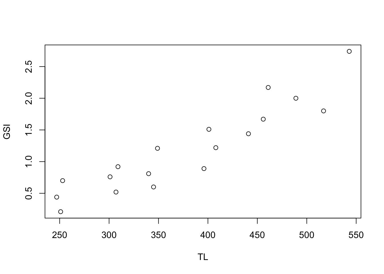Above is a simple scatter plot this plot was made with the code plot(GSI ~ TL), but could also be made with plot(TL, GSI).

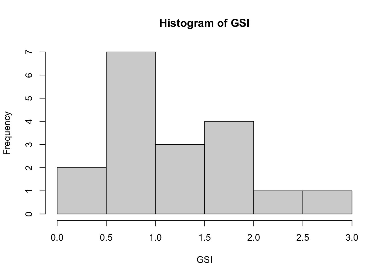Histograms are very useful, particularly in exploratory settings, to understand the shape or distribution of the frequency of values.

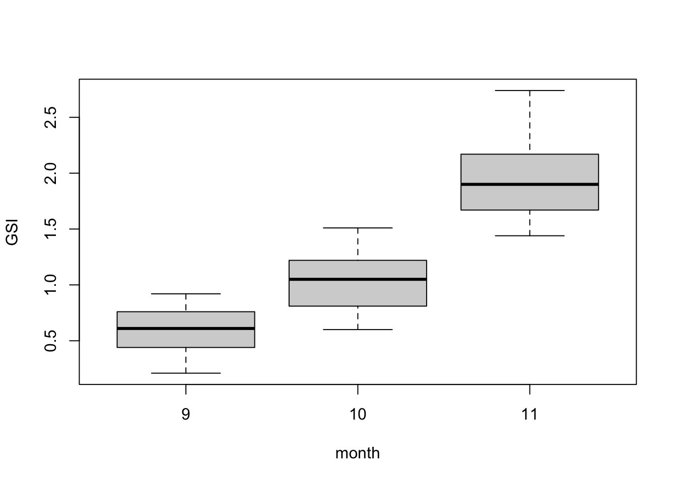Box plots are among the best ways to show normally-distributed numerical response data when it is split into different groups. In many instances, box plots should be used instead of bar plots.

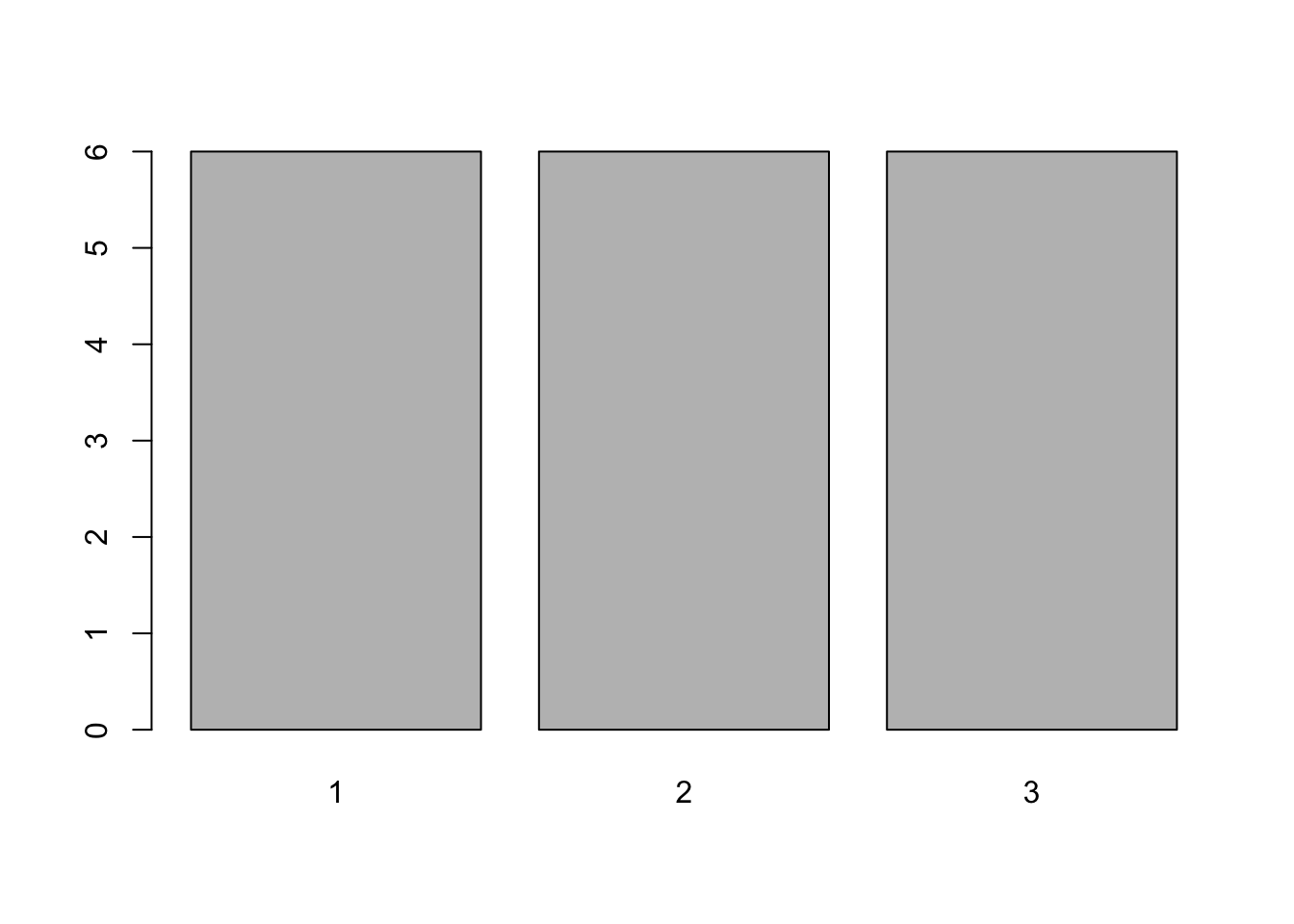Bar plot are good for showing counts, or other data that represents counts or accumulations with no variability. In the figure above, you need to tabulate the data first, and then use the bars to represent the tabulations. The figure above can be made with the simple code barplot(table(loc)).

Numerous other plot types are availble in base R, and even more with additional packages, but these four plots are very useful in a wide range of applications and are good to know.

2.7.2 Low-level Plotting

One thing you may have noticed is that the above plots may be correct, but they are not particularly visually appealing. To modify the formats, symbols, and other graphical elements, we we engage with low-level plotting.

Recall the scatterplot above that was created with only plot(GSI ~ TL). By changing some of the plot arguments, we can clean up the plot, make it more visually appealing, and also (hopefully) improve information transfer. The code below create the high-level plot, but then adds labels, changes symbol type, size, and color, and also rotates the y-axis label for improved readability.

plot(GSI ~ TL, # data to plot
  xlab = "Total length (mm)", # x-axis label
  ylab = "GSI (%)", # y-axis label
  main = "Southern Flounder GSI by TL", # main title
  pch = 19, # symbol
  cex = 1.5, # character expression (size; default = 1)
  col = "blue", # symbol color
  las = 1) # rotate y axis labels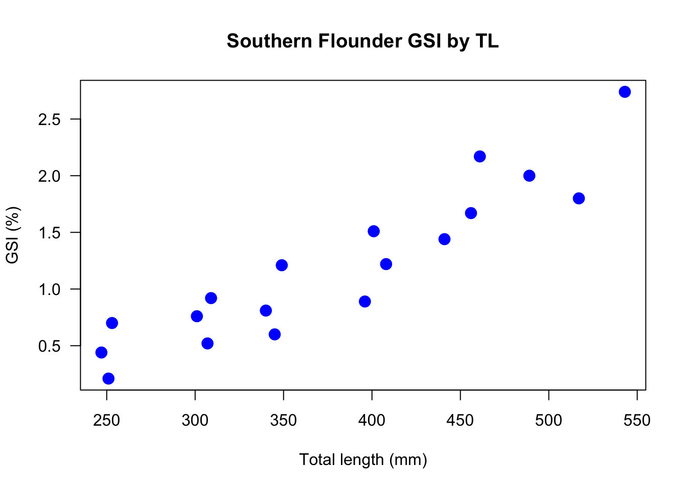

This is not a great plot, but it is already better than the first scatterplot of these data.

More low-level plotting can add more information.

plot(GSI ~ TL, # data to plot
  xlab = "Total length (mm)", # x-axis label
  ylab = "GSI (%)", # y-axis label
  main = "Southern Flounder GSI by TL", # main title
  pch = 19, # symbol
  col = loc, # colors (based on groups); c("red","blue","green")[loc]
  cex = 1.5, # character expression (size)
  las = 1) # rotate y axis labels
abline(a = lm(GSI~TL)$coefficients[1], b = lm(GSI~TL)$coefficients[2],
lwd = 3, lty = 2, col = "darkblue")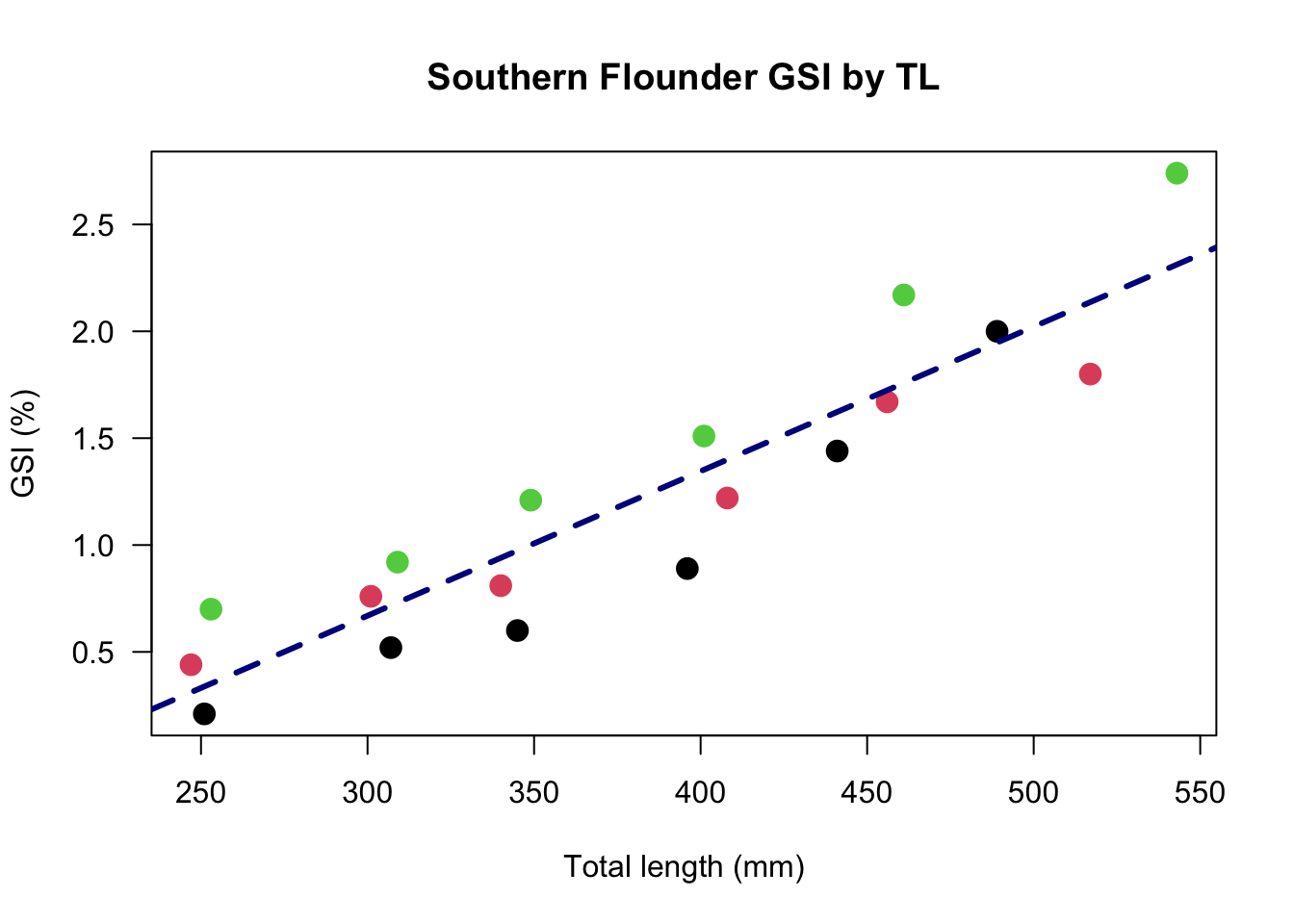

In the above figure, we have changed the color not to a specific color, but to reflect the location. (The location factors are interpreted alphabetically or numerically and assigned the default R color palette, where 1 = black, 2 = red, etc.) We have also added a line, using the abline() function. The a and b represent the intercept and slope, respectively, and can be specificed as numbers. Because we did not know these numbers of the top of our head, we stated that the intercept, a is the first coefficient produced by the linear model (lm()) of GSI regressed against TL. The slope is the second coefficient produced by that same model. We will cover all of this more in depth in the linear modeling chapter of this text, but this is just a brief explanation of how these numbers can be calcualted and plotted all in the same function.

Let’s improve the high-level boxplot shown above.

boxplot(GSI ~ month,
  range = 0, # extends whiskers to most extreme point
  varwidth = TRUE, # boxplot widths a function of group size
  #notch = TRUE, # quick visual significance
  col = "lightblue",
  border = "darkblue",
  las = 1,
  ylab = "GSI (%)",
  xaxt = "n" ) # remove x-axis
xlabs <- c("Sept", "Oct", "Nov")
axis(1, at = 9:11, labels = xlabs )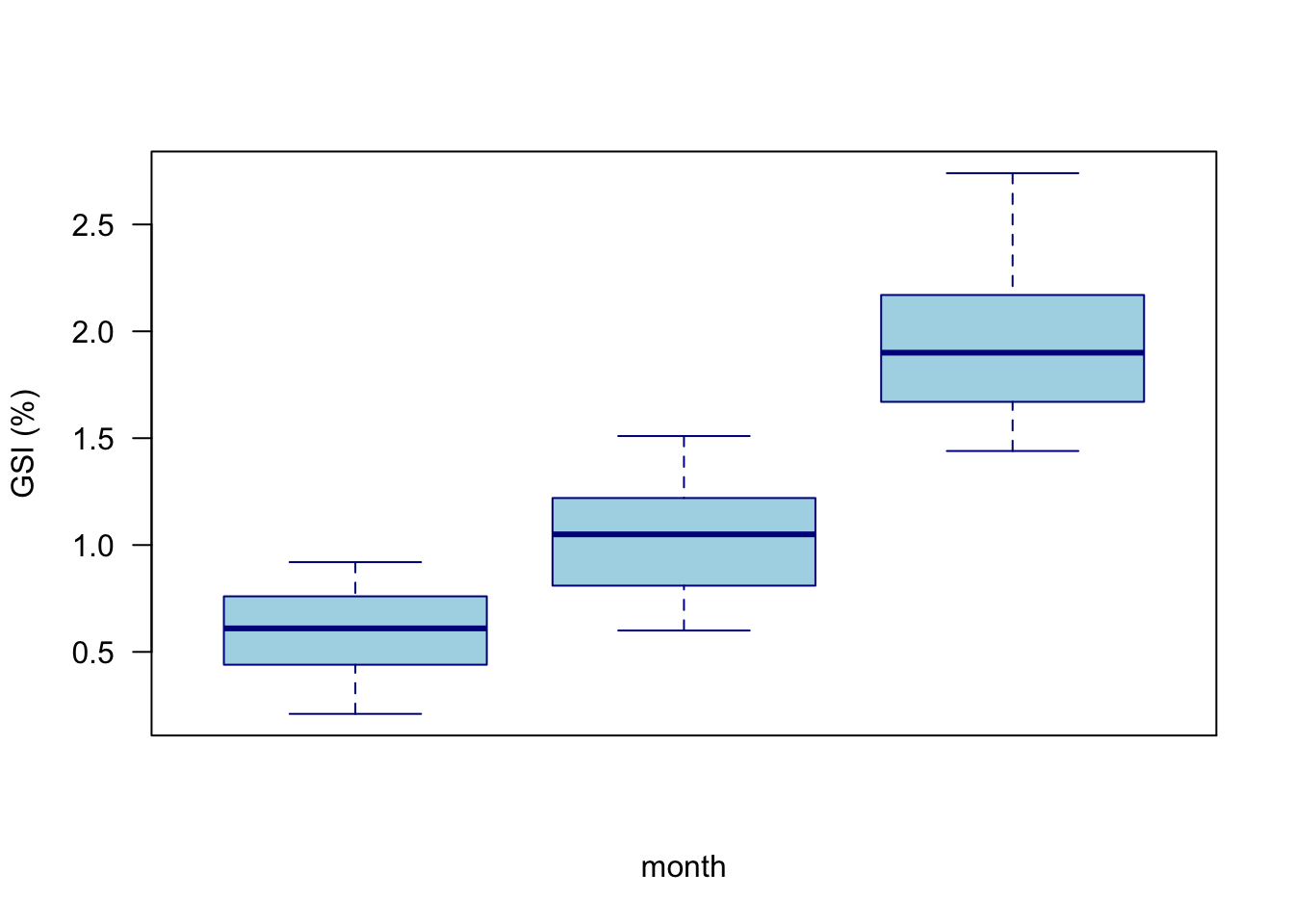

Of note here is that we did not want integer numbers for month labels. Although they were not wrong, it is more effective to use text. xaxt = "n" removes the default axes, and we then add a function to define the text labels we want, followed by the axis() command to add those custom labels to the plot. See ?axis for details on how to specify custom axes.

2.7.3 Plotting Panels

You may want to create small multiples of plots, whereby some plot type is repeated for different groupings of the data. Although there are numerous ways to accomplish this, one simple approach is to use the lattice library and the xyplot() function.

In the code below, we load the library, and use the xyplot() function to specify the GSI and TL relationship we want, but in this case is followed by | loc, which means we specifies separate panels for each location. The "p" and "r" tell the function we want points and a regression line to be included.

library(lattice)
xyplot(GSI ~ TL | loc, # Group by location
  type = c("p","r"), # Add regression line
  pch = 19, cex = 1.5)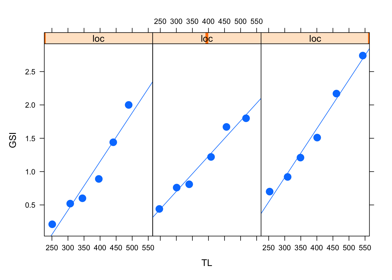

ggplot2 and other packages have excellent functions for paneling plots and these other packages may be ultimately recommended. But remember the goal here is simple fluency and execution, often for exploratory purposes.

2.7.4 Graphical Parameters

Although you cannot often see it, your plot object is being placed on a layout with certain defaults. As you include multiple plots or panels into one layout, you may need to change margin sizes and other graphical parameters. Graphical flexibility is extensive; however, it can take some research and trial and error for custom layouts. Most commonly, you will need to modify the outer margins oma(), (inner) margins mar(), and the rows mfrow() and columns mfcol() within the layout.

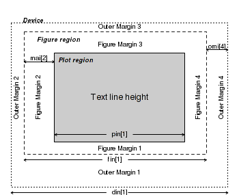
Figure 2.1: Graphical layout

Note that the oma(), mar(), and other functions are used within the par() environment. Text is also easily added at the x and y coordinates you specify in the text() function.

par(
oma(3,3,2,1) # c(bottom, left, top, right) for outer margins
mar(3,3,2,1) # c(bottom, left, top, right) for plot margins
mfrow(3,2) # panel of 3 rows, 2 columns
mfcol(3,2) # panel of 3 columns, 2 rows
)

#Add text
text(x, y, "Some informative text")

2.8 Other Resources for Learning R

As stated earlier in this chapter, the content presented here is not intended to be comprehensive or a singular source for learning R. Honestly, most people learn R through coding something they need to do and in making and solving a lot of mistakes. But in addition to that on-the-job-training, there are a number of good resources for learning R, and because everyone learns a little differently, you are encouraged to check out as many R resources as you can. The resources presented below are neither comprehensive, nor specifically endorsed, and are only included because they have been recommended by others. Note that resources range from free to paid.

2.8.1 Online Interactive Training

2.8.2 R Packages

swirl
learnr

2.8.3 Books

2.8.4 Websites

…and, of course, Google it!

Figure 2.2: Source: XKCD