7 Overview of statistical methods
7.1 Introduction to spatial modelling
The first law of geography (Tobler, 1970) states that areas near each other are likely to be more similar to each other than areas further away. Spatial modelling is motivated by this law because it implies that we can gain information about an area from its neighbours. It also underpins our approach, which is to use information on the spatial structure of Australia to improve estimates for each small area.
The geographical estimates reported in the Australian Cancer Atlas were generated by fitting statistical models, called Bayesian spatial models, to data that includes geographical location. (Kang et al., 2016) Bayesian modelling is a flexible form of statistical modelling that provides readily interpretable information about the uncertainty of the results. Spatial models consider the geographical structure of the data. For a comprehensive description of Bayesian statistics and spatial models, please refer to our e-book. (Duncan et al., 2019b)
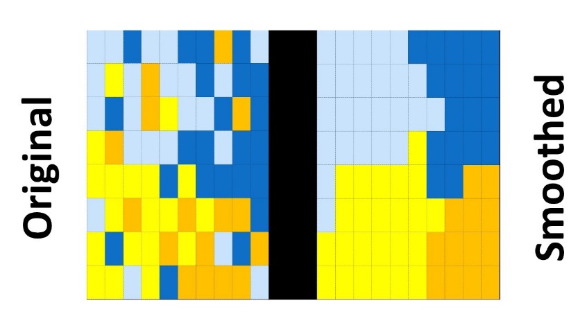
Bayesian spatial modelling smooths rates by ‘borrowing’ information from neighbouring geographical areas. Spatial smoothing is important in providing estimates of the cancer burden for small areas for three reasons. Firstly, it reduces the risk of identifying individual people. Secondly, it improves the stability of the resulting estimates, which can fluctuate for uncommon conditions like cancer. Thirdly, it can provide evidence that any differences are real and not just due to chance. (Cramb et al., 2016) A typical (but hypothetical) impact that smoothing can have on observed geographical data is shown in Figure 7.1.
There are numerous ways to define how the neighbouring areas contribute to spatial smoothing. Spatial information can be incorporated as the distance between areas or as adjacency information. The Australian Cancer Atlas used adjacency information and areas were deemed to be adjacent to each other if they shared a boundary. The models used stated that each area’s estimates depended on the estimates of the adjacent areas, making the estimate similar to those of its neighbours. Details of the adjacency structure and overall model formulation are given below. Specific details for the different models used for each of the indicators are given in Sections 8 to 12.
7.1.1 Spatial models (all indicators except risk factors)
The Australian Cancer Atlas used Bayesian spatial models to estimate the geographical patterns (relative to Australian average) over aggregated time periods for each included indicator. The results of these spatial models can be seen if the “type of estimate” selected is “Geographical patterns (average)”. There are a range of Bayesian spatial models available that differ for example in how neighbours are defined, the type of smoothing applied and other aspects of the model specification. All models used for the Atlas belong to a class of spatial models termed “Conditional Autoregressive (CAR) models”. (Cramb et al., 2016) These models incorporate the first law of geography by assuming that an area’s rates are similar to the average of the adjoining geographical areas. Bayesian models also provide a probabilistic description for each of the unknown parameters, which is helpful in quantifying the extent of uncertainty around the spatial estimates.
The model employed for modelling cancer diagnoses for the Australian Cancer Atlas was selected based on a rigorous process of testing and evaluation of spatial models. During this process, a variety of relevant models were compared using a range of criteria including the plausibility of estimates, computational time, and feasibility. (Cramb et al., 2018, Cramb et al., 2020) Spatial models for other indicators reported in the Atlas were also chosen based on a similar process.
All models included spatial random effects terms to incorporate information about nearest neighbours and generate smoothed estimates. Models for cancer diagnosis (Section 8.4.2), screening or testing (Sections 11.1.2.2, 11.2.2.2, 11.3.2.2, 11.4.2.2) and hospital treatment (Section 12.3.2) were based on aggregated count data. The selected model started with the likelihood model for the observed count data, with the expected counts based on national age-specific rates, then included an intercept term and a spatial random effect for each area. For cancer survival, a Poisson spatial survival model was used, that included various covariates (broad age group, sex, and cancer type) and follow-up time up to five years since diagnosis. Further details are in Section 9.4.3.
7.1.2 Spatiotemporal models
For many cancer types, geographical patterns have changed over time. To understand the changes, we used spatiotemporal models that describe variation by geographical area and time. The spatiotemporal estimates can be seen if the “type of estimate” selected is either “Geographical patterns (separate time periods)” or “Changes over time for each geographical area”. The estimates for each type of estimate are presented as a series of maps, one map for each time point.
Two types of spatiotemporal estimates are available from the Australian Cancer Atlas. The first type shows the geographic patterns for each time period separately. In each map, the areas’ rates are compared to the Australian average for the time period of the map shown. This means that for each time period, some areas’ rates will be above average and some below average.
The second type of estimate shows how areas’ rates compare with the Australian average for all time periods available. This means that if rates are increasing or decreasing across Australia, many areas may have above average rates at certain time points and at other time points most areas may have below average rates.
The spatiotemporal models for cancer diagnosis in the Australian Cancer Atlas were based on the model of Bernardinelli and colleagues (Bernardinelli et al., 1995) and the design of the temporal trends on the work of Crainiceanu and colleagues. (Crainiceanu et al., 2005)These models described the interaction between time and space by including a national temporal trend, area-specific effects, and area-specific deviations from the national trend. Further details are in Sections 8.4.3 for diagnosis models, 9.4.5 for survival models and 12.3.3 for hospital treatment models.
7.1.3 Survey estimation (cancer risk factors)
Because the risk factor data came from survey data, a newly developed Bayesian two-stage small area estimation approach was used to obtain risk factor estimates by SA2. (Hogg et al., 2023)
In the first stage, we used a hierarchical Bayesian logistic model on individual-level 2017-18 National Health Survey data. This model included various health, and socio-demographic factors, in addition to SA2-level socioeconomic status. The probabilities from the first stage model were used to calculate weighted prevalence estimates for SA2 areas with survey data.
In the second stage, the previously generated prevalence estimates were smoothed further using a Bayesian spatial model. This second stage model produced prevalence estimates for all SA2s included in the modelling (2,221 SA2 areas). This model included random effects at the SA2 and Statistical Area Level 3 (SA3) levels, SA2-level covariates (such as socioeconomic data), and previously published risk factor prevalence estimates from the Social Health Atlas of Australia. (Social Health Atlas) More details are in Section 10.3.2.
7.1.4 Neighbourhood structure
For a specific area, the neighbours were defined as those SA2s having a shared boundary of any length and an estimated annual resident population of at least five people. There were additional refinements made to this default definition for the Australian Cancer Atlas. The 13 island areas lacking neighbours were each assigned at least one neighbour, and often this was the closest mainland area. This neighbourhood structure was then represented in a matrix, called an ‘adjacency matrix’. Note that symmetry was required in the adjacency matrix, so that any area with a specific area assigned as a neighbour was also assigned to be the neighbour of that area. The adjacency matrix used can be provided on request. (atlas@cancerqld.org.au)
For the cancer risk factor modelling, a different adjacency matrix was used to induce more smoothing. For these models, donut SA2s, or areas with only one neighbour (n = 87), were also assigned the neighbours of their neighbour. The final adjacency matrix assigned 93% of SA2s more than two neighbours. Furthermore, the eastern and western SA2s at the top of Tasmania were considered as neighbours of the furthest south SA2s in Victoria.
7.1.5 Computation
Popular approaches to fitting Bayesian spatial models include simulation methods such as Markov Chain Monte Carlo (MCMC) or approximation methods such as integrated nested Laplace approximation or Variational Bayes. (Cramb et al., 2016) For the Australian Cancer Atlas, we have used the MCMC approach, because it provides greater information about the uncertainty of the estimates and better model fits.
Models were implemented in R (https://www.R-project.org/) using the CARBayes package, (Lee, 2021) WinBUGS, (Lunn et al., 2000) the R2WinBUGS package, (Sturtz et al., 2015) Nimble, (de Valpine et al., 2017) and Stan. (https://mc-stan.org)
7.1.6 Assessing convergence
Convergence was assessed through visual examination of trace and density plots for a subset of parameters and areas as well as estimating the effective sample size and \(\widehat{R}\). (Aki et al., 2021) The Geweke (Geweke, 1992) diagnostic for the modelled estimates was examined for all areas. Areas with a Geweke p-value <0.01 were flagged and examined visually.
7.1.7 Sensitivity analyses
Examining the influence of the priors is an essential part of any Bayesian analysis. Of greatest concern in these models are the priors on the variance component of the prior (i.e. the hyperpriors). Priors for the spatial models for cancer diagnosis and cancer survival in Australian Cancer Atlas 2.0 were based on the previous sensitivity analysis carried out for Atlas 1.0. (Duncan et al., 2019a)
Sensitivity analysis showed that the models for cancer screening, (Dasgupta et al., 2023b) testing, (Kohar et al., 2023) and hospital treatment (Cameron et al., 2023) were not sensitive to the choice of priors or hyperpriors.
7.1.8 Software used
Stata, R, WinBUGS and Stan software were used in the creation of the modelled estimates reported in the Australian Cancer Atlas 2.0.
Initial data manipulation and calculation of national summary measures was performed using Stata v17.0 (StataCorp, Texas), as follows:
National age-standardised rates using the ‘distrate’ command (Coviello, 2006)
Relative survival using the ‘strs’ command (Dickman and Coviello, 2015)
All adjacency matrixes were created using R. WinBUGS v1.4.3 interfaced with R was used to run the Bayesian spatial survival models. For the Bayesian cancer risk factor models, Stan was interfaced with R using rstan v2.26.11. All other analyses used R.
7.1.9 Uncertainty of modelled estimates
The colours in the maps of the Australian Cancer Atlas are based on the best estimate of the areas’ rates compared with the Australian average. However, each estimate has a degree of uncertainty, or imprecision, around it. Areas with smaller populations, such as SA2s, generally have greater uncertainty around their estimates.
In the Australian Cancer Atlas, two aspects of uncertainty are presented:
The uncertainty of each SA2s estimate and
The uncertainty that the estimate for a given SA2 is statistically different from the national average.
The first aspect relates to the precision of an estimate and is portrayed using wave plots and credible intervals in the Australian Cancer Atlas. These appear under the colour bar and V-plot when an area is selected. The MCMC simulations (see Section 7.1.5) produce thousands of possible values for each area. If these values are ordered from smallest estimate to largest, the middle value (that is, the median or 50th quantile) is the value displayed on the maps. The credible intervals describe the range of estimates that are more plausible than others. For example, 80% of the MCMC estimates lie between the values of the 80% credible interval, which is calculated as the 10th and 90th quantiles. The 60% and 80% credible intervals are displayed as unfilled and filled circles (respectively) under the wave plot. The distribution of the MCMC simulations is summarised visually by the “wave plot”, described in more detail in Section 14.3.1 along with screenshots.
The second aspect of the uncertainty relates to the evidence that an area’s estimate is different to the Australian average. For spatial diagnosis models, for example, the estimated standardised incidence ratio (SIR) for a given area is interpreted as the risk of being diagnosed relative to the Australian average risk. By calculating the proportion of MCMC samples for the SIR that were greater than one, we can compute the probability of an area’s estimate being above or below one. Specifically, the exceedance probability (\(EP\)) of an area’s estimate being greater than one is given by:
\[{EP}_{i} = \frac{1}{M}\sum_{m = 1}^{M}{\prod_{}^{}\left( A_{i}^{(m)}\ > 1\ \right)}\]
where Ai(m) is the mth MCMC estimate for area i.
The \(EP_{i}\) is used in the Comparison view (see Section 14.10), where an area with an \(EP_{i}\) less than 0.2 was classed as “low”, an area with an \(EP_{i}\) greater than 0.8 was classed as “high” and an area with an \(EP_{i}\) between 0.2 and 0.8 was classed as “average”, based on the work of Richardson and colleagues. (Richardson et al., 2004)
By symmetry, the probability that area i’s estimate is less than or equal to one is:
\[{EP}_{i,\ below} = 1 - {EP}_{i}\]
A new measure was constructed, the posterior probability difference (PPD), which represents the evidence that the SIR is different from one.
\[PPD_{i} = \ \left| EP_{i} - EP_{i,below} \right|\]
The PPD is shown in the “V-plot” and it also forms the basis of the “transparency” feature in the Australian Cancer Atlas.
Note that for some spatiotemporal estimates, the interpretation is slightly different. If the type of estimate selected is “Changes over time for each geographical area”, the PPD provides evidence that an area’s rate is different to the national average, where the national average was calculated over all the time periods available.
Details of how these measures of uncertainty are visualised in the Atlas are described in Section 14.3.2 and 14.3.3.