9 Tabular Data

9.1 Test of proportions

Many times, we are interested in estimating and inference on the proportion \(p\) in a Bernoulli trial. For example, we may be interested in the true proportion of times that a die shows a 6 when rolled, or the proportion of voters in a population who favor a particular candidate. In order to do this, we will run \(n\) trials of the experiment and count the number of times that the event in question occurs, which we denote by \(x\). For example, we could toss the die \(n = 100\) times and count the number of times that a 6 occurs, or sample \(n = 500\) voters (from a large population) and ask them whether they prefer a particular candidate. Note that in the second case, this is not formally a Bernoulli trial unless you allow the possibility of asking the same person twice; however, if the population is large, then it is approximately repeated Bernoulli trials.

The natural estimator for the true proportion \(p\) is given by \[ \hat p = \frac xn \] However, we would like to be able to form confidence intervals and to do hypothesis testing with regards to \(p\). Here, we present the theory associated with performing exact binomial hypothesis tests using binom.test, as well as prop.test, which uses the normal approximation.

9.1.1 Hypothesis Testing

Suppose that you have null hypothesis \(H_0: p = p_0\) and alternative \(H_a: p \not= p_0\). You run \(n\) trials and obtain \(x\) successes, so your estimate for \(p\) is given by \(\hat p = x/n\). Presumably, \(\hat p\) is not exactly equal to \(p_0\), and you wish to determine the probability of obtaining an estimate that far away from \(p_0\) or further. Formally, we are going to add the probabilities of all outcomes that are no more likely than the outcome that was obtained, since if we are going to reject when we obtain \(x\) successes, we would also reject if we obtain a number of successes that was even less likely to occur.

Example (Using binom.test) Suppose you wish to test \(H_0: p = 0.4\) versus \(H_a: p \not= 0.4\). You do 100 trials and obtain 50 successes.The probability of getting exactly 50 successes is dbinom(50, 100, 0.4), or 0.01034. Anything more than 50 successes is less likely under the null hypothesis, so we would add all of those to get part of our \(p\)-value. To determine which values we add for successes less than 40, we look for all outcomes that have probability of occurring (under the null hypothesis) less than 0.01034. Namely, those are the outcomes between 0 and 30, since dbinom(30, 100, 0.4) is 0.1001. See also the following figure, where the dashed red line indicates the likelihood of observing exactly 50 successes. We sum all of the probabilities that are below the dashed red line. (Note that the x-axis has been truncated.)

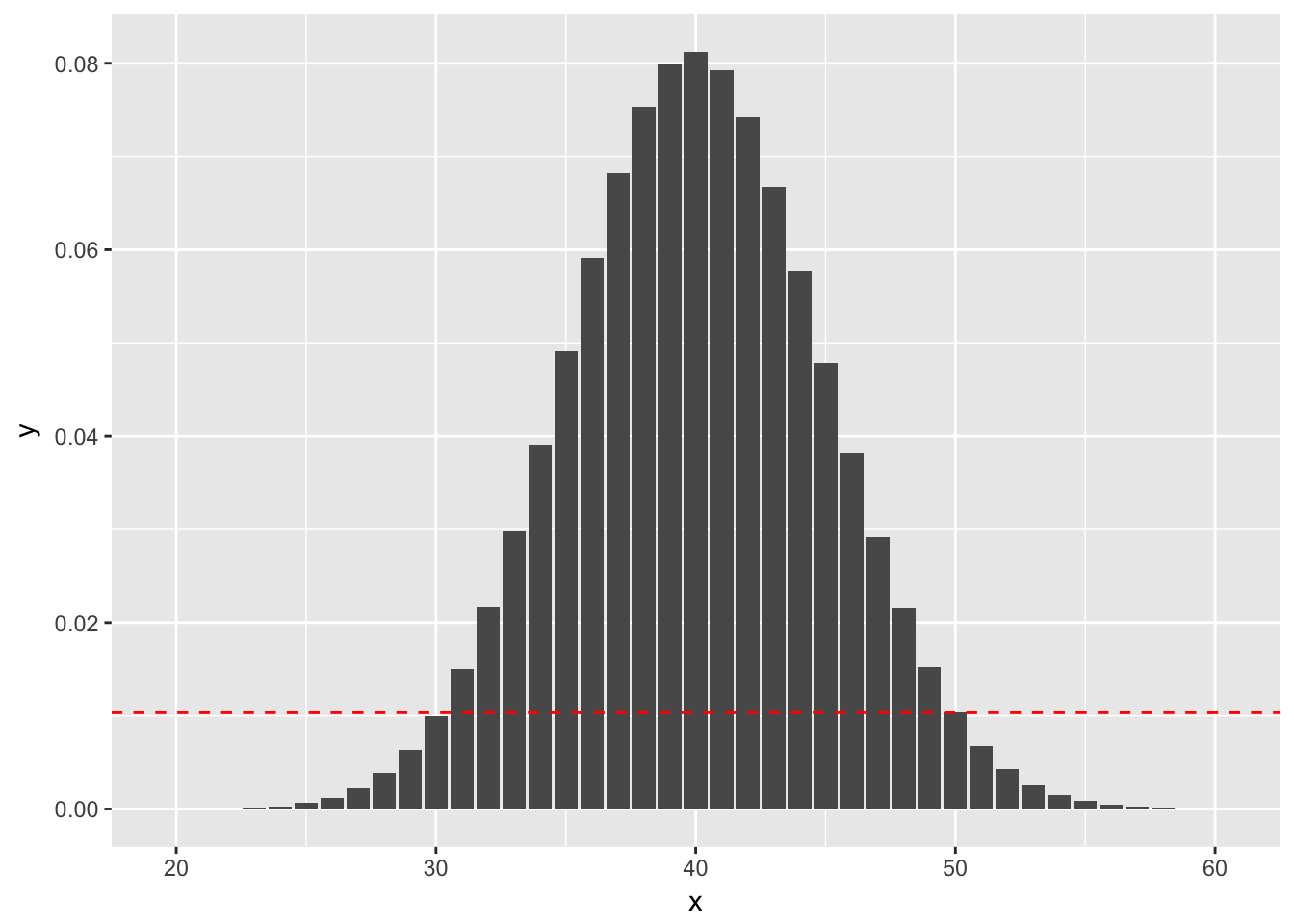
So, the \(p\)-value would be \[ P(X \le 30) + P(X \ge 50) \] where \(X\sim\) Binomial(n = 100, p = 0.4).

sum(dbinom(x = 50:100, size = 100, prob = .4)) + sum(dbinom(x = 0:30, size = 100, prob = .4))

## [1] 0.05188202

On the other hand, if we obtained 30 successes, the \(p\)-value would sum the probabilities that are less than observing exactly 30 successes, as indicated by this plot:

ggplot(plotData, aes(x, y)) + geom_bar(stat = "identity") +
  geom_abline(slope = 0, intercept = dbinom(30, 100, 0.4), linetype = "dashed", color = "red")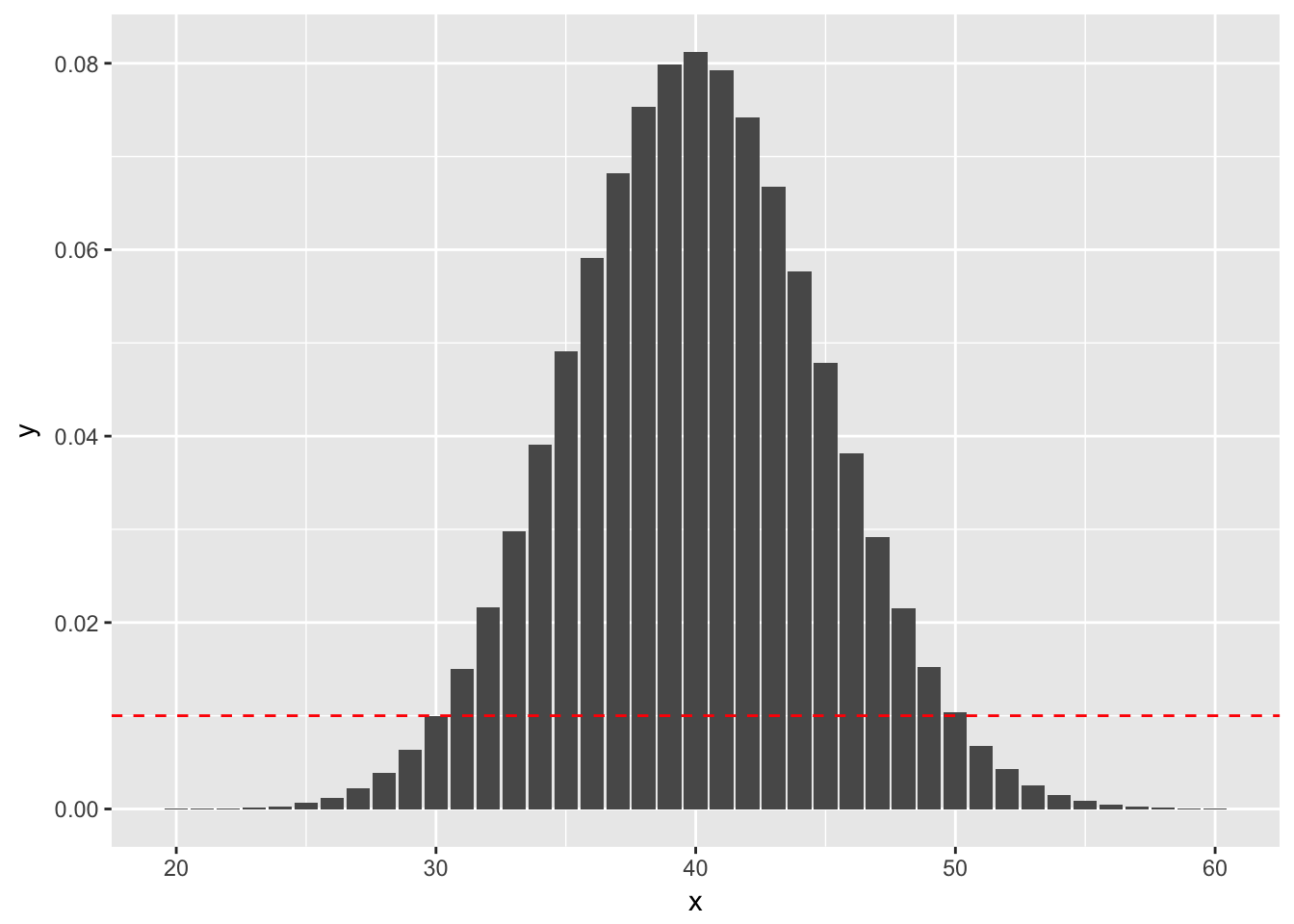

sum(dbinom(x = 51:100, size = 100, prob = .4)) + sum(dbinom(x = 0:30, size = 100, prob = .4))

## [1] 0.04154451

because the outcomes that are less likely under the null hypothesis than obtaining 30 successes are (1) getting fewer than 30 successes, and (2) getting 51 or more successes. Indeed, dbinom(51, 100, 0.4) is 0.0068.

R will make these computations for us, naturally, in the following way.

binom.test(x = 50, n = 100, p = .4)

## 
##  Exact binomial test
## 
## data:  50 and 100
## number of successes = 50, number of trials = 100, p-value =
## 0.05188
## alternative hypothesis: true probability of success is not equal to 0.4
## 95 percent confidence interval:
##  0.3983211 0.6016789
## sample estimates:
## probability of success 
##                    0.5

binom.test(x = 30, n = 100, p = .4)

## 
##  Exact binomial test
## 
## data:  30 and 100
## number of successes = 30, number of trials = 100, p-value =
## 0.04154
## alternative hypothesis: true probability of success is not equal to 0.4
## 95 percent confidence interval:
##  0.2124064 0.3998147
## sample estimates:
## probability of success 
##                    0.3

Example (Using prop.test) When \(n\) is large and \(p\) isn’t too close to 0 or 1, binomial random variables with \(n\) trials and probability of success \(p\) can be approximated by normal random variables with mean \(np\) and standard deviation \(\sqrt{np(1 - p)}\). This can be used to get approximate \(p\)-values associated with the hypothesis test \(H_0: p = p_0\) versus \(H_a: p\not= p_0\).

We consider again the example that in 100 trials, you obtain 50 successes when testing \(H_0: p = 0.4\) versus \(H_a: p\not= 0.4\). Let \(X\) be a binomial random variable with \(n = 100\) and \(p = 0.4\). We approximate \(X\) by a normal rv \(N\) with mean \(np = 40\) and standard deviation \(\sqrt{np(1 - p)} = 4.89879\). As before, we need to compute the probability under \(H_0\) of obtaining an outcome that is as likely or less likely than obtaining 50 successes. However, in this case, we are using the normal approximation, which is symmetric about its mean. Therefore, the \(p\)-value would be \[ P(N \ge 50) + P(N \le 30) \] We compute this via

pnorm(50, 40, 4.89879, lower.tail = FALSE) + pnorm(30, 40, 4.89879)

## [1] 0.04121899

The built in R function for this is prop.test, as follows:

prop.test(x = 50, n = 100, p = 0.4, correct = FALSE)

## 
##  1-sample proportions test without continuity correction
## 
## data:  50 out of 100, null probability 0.4
## X-squared = 4.1667, df = 1, p-value = 0.04123
## alternative hypothesis: true p is not equal to 0.4
## 95 percent confidence interval:
##  0.4038315 0.5961685
## sample estimates:
##   p 
## 0.5

Note that to get the same answer as we did in our calculations, we need to set correct = FALSE. It is typically desirable to set correct = TRUE, which performs a continuity correction. The basic idea is that \(N\) is a continuous rv, so when \(N = 39.9\), for example, we need to decide what integer value that should be associated with. Continuity corrections do this in a way that gives more accurate approximations to the underlying binomial rv (but not necessarily closer to using binom.test).

prop.test(x = 50, n = 100, p =  .4)

## 
##  1-sample proportions test with continuity correction
## 
## data:  50 out of 100, null probability 0.4
## X-squared = 3.7604, df = 1, p-value = 0.05248
## alternative hypothesis: true p is not equal to 0.4
## 95 percent confidence interval:
##  0.3990211 0.6009789
## sample estimates:
##   p 
## 0.5

9.1.2 Confidence Intervals

Confidence intervals for \(p\) can be read off of the output of the binom.test or prop.test. They again will give slightly different answers. We illustrate the technique using prop.test.

Example The Economist/YouGov poll leading up to the 2016 presidential election sampled 3669 likely voters and found that 1798 intended to vote for Clinton. Assuming that this is a random sample from all likely voters, find a 99% confidence interval for \(p\), the true proportion of likely voters who intended to vote for Clinton at the time of the poll.

prop.test(x = 1798, n = 3699, conf.level = 0.99)

## 
##  1-sample proportions test with continuity correction
## 
## data:  1798 out of 3699, null probability 0.5
## X-squared = 2.8127, df = 1, p-value = 0.09352
## alternative hypothesis: true p is not equal to 0.5
## 99 percent confidence interval:
##  0.4648186 0.5073862
## sample estimates:
##         p 
## 0.4860773

Thus, we see that we are 99% confident that the true proportion of likely Clinton voters was between .4648186 and .5073862. (Note that in fact, 48.2% of the true voters did vote for Clinton, which does fall in the 99% confidence interval range.)

9.2 \(\chi^2\) tests.

9.3 Exercises

(Hard) Suppose you wish to test whether a die truly comes up “6” 1/6 of the time. You decide to roll the die until you observe 100 sixes. You do this, and it takes 560 rolls to observe 100 sixes.
1. State the appropriate null and alternative hypotheses.
2. Explain why prop.test and binom.test are not formally valid to do a hypothesis test.
3. Use reasoning similar to that in the explanation of binom.test above and the function dnbinom to compute a \(p\)-value.
4. Should you accept or reject the null hypothesis?