11 Analysis of Variance
In this chapter, we introduce one-way analysis of variance (ANOVA) through the analysis of a motivating example.
Consider the red.cell.folate data in ISwR. We have data on folate levels of patients under three different treatments. Suppose we want to know whether treatment has a significant effect on the folate level of the patient. How would we proceed?
First, we would want to plot the data. A boxplot is a good idea.
red.cell.folate <- ISwR::red.cell.folate
ggplot(red.cell.folate, aes(x = ventilation, y = folate)) +
  geom_boxplot()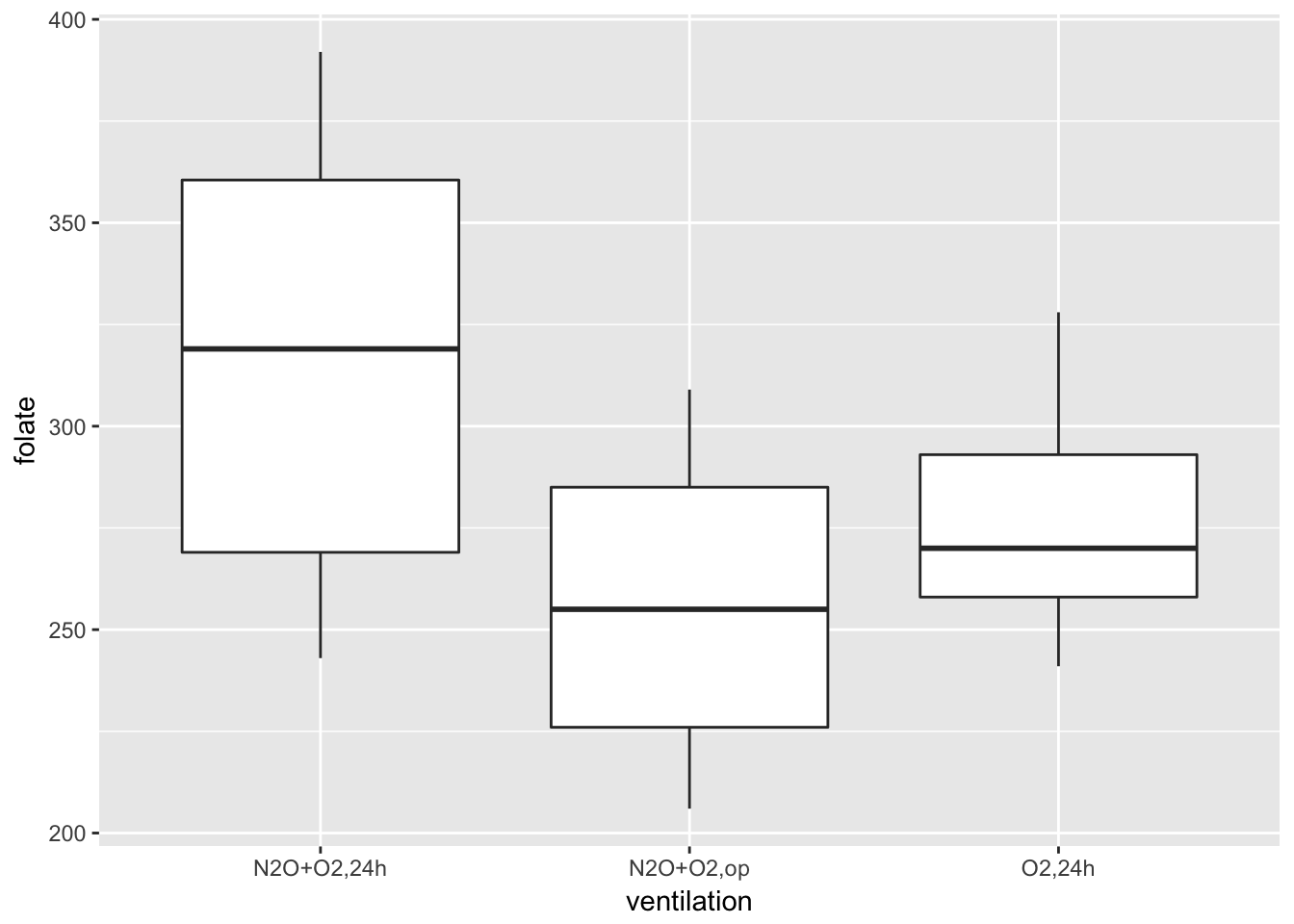
Looking at this data, it is not clear whether there is a difference. It seems that the folate level under treatment 1 is perhaps higher. We could try to compare the means of each pair of ventilations using t.test(). The problem with that is we would be doing three tests, and we would need to adjust our \(p\)-values accordingly. We are going to take a different approach, which is ANOVA.
11.1 Setup
Notation
- \(x_{ij}\) denotes the \(j\)th observation from the \(i\)th group.
- \(\overline{x}_{i\cdot}\) denotes the mean of the observations in the \(i\)th group.
- \(\overline{x}_{\cdot}\) denotes the mean of all observations.
As an example, in red.cell.folate, there are 3 groups. We have \(x_{11} = 243, x_{12} = 251, \ldots, x_{21} = 206,\ldots,x_{31} = 241,\ldots.\)
To compute the group means:
red.cell.folate %>% group_by(ventilation) %>% summarize(mean(folate))## # A tibble: 3 x 2
## ventilation `mean(folate)`
## <fctr> <dbl>
## 1 N2O+O2,24h 316.6250
## 2 N2O+O2,op 256.4444
## 3 O2,24h 278.0000This tells us that \(\overline{x}_{1\cdot} = 316.625\), for example.
To get the overall mean, we use mean(red.cell.folate$folate), which is 283.2.
Our model for the folate level is \[ x_{ij} = \mu + \alpha_i + \epsilon_{ij}, \] where \(\mu\) is the grand mean, \(\alpha_i\) represents the difference between the grand mean and the group mean, and \(\epsilon_{ij}\) represents the variation within the group. So, each individual data point could be realized as \[ x_{ij} = \overline{x}_\cdot + (\overline{x}_{i\cdot} - \overline{x}) + (x_{ij} - \overline{x}_{i\cdot}) \]
The null hypothesis for ANOVA is that the group means are all equal (or equivalently all of the \(\alpha_i\) are zero). So, if \(\mu_i = \mu + \alpha_i\) is the true group mean, we have:
\[ H_0 : \mu_1 = \mu_2 = \cdots =\mu_k\\ H_a : \text{Not all $\mu_i$ are equal} \]
11.2 ANOVA
ANOVA is “analysis of variance” because we will compare the variation of data within individual groups with the overall variation of the data. We make assumptions (below) to predict the behavior of this comparison when \(H_0\) is true. If the observed behavior is unlikely, it gives evidence against the null hypothesis. The general idea of comparing variance within groups to the variance between groups is applicable in a wide variety of situations.
Define the variation within groups to be \[ SSD_W = \sum_i \sum_j (x_{ij} - \overline{x}_{i\cdot})^2 \] and the variation between groups to be \[ SSD_B = \sum_i\sum_j (\overline{x}_{i\cdot} - \overline{x})^2 \] and the total variation to be \[ SSD_{tot} = \sum_i \sum_j (\overline{x} - x_{ij})^2. \]
This says that the total variation can be broken down into the variation between groups plus the variation within the groups. If the variation between groups is much larger than the variation within groups, then that is evidence that there is a difference in the means of the groups. The question then becomes: how large is large? In order to answer that, we will need to examine the \(SSD_B\) and \(SSD_W\) terms more carefully. At this point, we also will need to make
Assumptions
- The population is normally distributed within each group
- The variances of the groups are equal. (Yikes!)
Notation We have \(k\) groups. There are \(n_i\) observations in group \(i\), and \(N = \sum n_i\) total observations.
Notice that \(SSD_W\) is almost \(\sum\sum (\overline{x}_{ij} - \mu_i)^2\), in which case \(SSD_W/\sigma^2\) would be a \(\chi^2\) random variable with \(N\) degrees of freedom. However, we are making \(k\) replacements of means by their estimates, so we subtract \(k\) to get that \(SSD_B/\sigma^2\) is \(\chi^2\) with \(N - k\) degrees of freedom. (This follows the heuristic we started in Section 4.6.2).
As for \(SSD_B\), it is trickier to see, but \(\sum_i \sum_j (x_{i\cdot} - \mu)^2/\sigma^2\) would be \(\chi^2\) with \(k\) degrees of freedom. Replacing \(\mu\) by \(\overline{x}\) makes \(SSD_B/\sigma^2\) a \(\chi^2\) rv with \(k - 1\) degrees of freedom.
The test statistic for ANOVA is: \[ F = \frac{SSD_B/(\sigma^2(k - 1))}{SSD_W/(\sigma^2(N - k))} = \frac{SSD_B/(k - 1)}{SSD_W/(N - k)} \]
This is the ratio of two \(\chi^2\) rvs divided by their degrees of freedom; hence, it is \(F\) with \(k - 1\) and \(N - k\) degrees of freedom. Through this admittedly very heuristic derivation, you can see why we must assume that we have equal variances (otherwise we wouldn’t be able to cancel the unknown \(\sigma^2\)) and normality (so that we get a known distribution for the test statistic).
If \(F\) is much bigger than 1, then we reject \(H_0: \mu_1 = \mu_2 = \cdots =\mu_k\) in favor of the alternative hypothesis that not all of the \(\mu_i\) are equal.
11.3 Examples
11.3.1 red.cell.folate
Returning to red.cell.folate, we use R to do all of the computations for us.
First, build a linear model for folate as explained by ventilation, and then apply the anova function to the model. anova produces a table which contains all of the computations from the discussion above.
rcf.mod <- lm(folate~ventilation, data = red.cell.folate)
anova(rcf.mod)
## Analysis of Variance Table
##
## Response: folate
## Df Sum Sq Mean Sq F value Pr(>F)
## ventilation 2 15516 7757.9 3.7113 0.04359 *
## Residuals 19 39716 2090.3
## ---
## Signif. codes: 0 '***' 0.001 '**' 0.01 '*' 0.05 '.' 0.1 ' ' 1The two rows ventilation and Residuals correspond to the between group and within group variation.
The first column, Df gives the degrees of freedom in each case. Since \(k = 3\), the between group variation has \(k - 1 = 2\) degrees of freedom, and since \(N = 22\), the within group variation (Residuals) has \(N - k = 19\) degrees of freedom.
The Sum Sq column gives \(SSD_B\) and \(SSD_W\). The Mean Sq variable is the Sum Sq value divided by the degrees of freedom. These two numbers are the numerator and denominator of the test statistic, \(F\). So here, \(F = 7757.9/2090.3 = 3.7113\).
To compute the \(p\)-value, we need the area under the tail of the \(F\) distribution above \(F = 3.7113\). Note that this is a one-tailed test, because small values of \(F\) would actually be evidence in favor of \(H_0\).
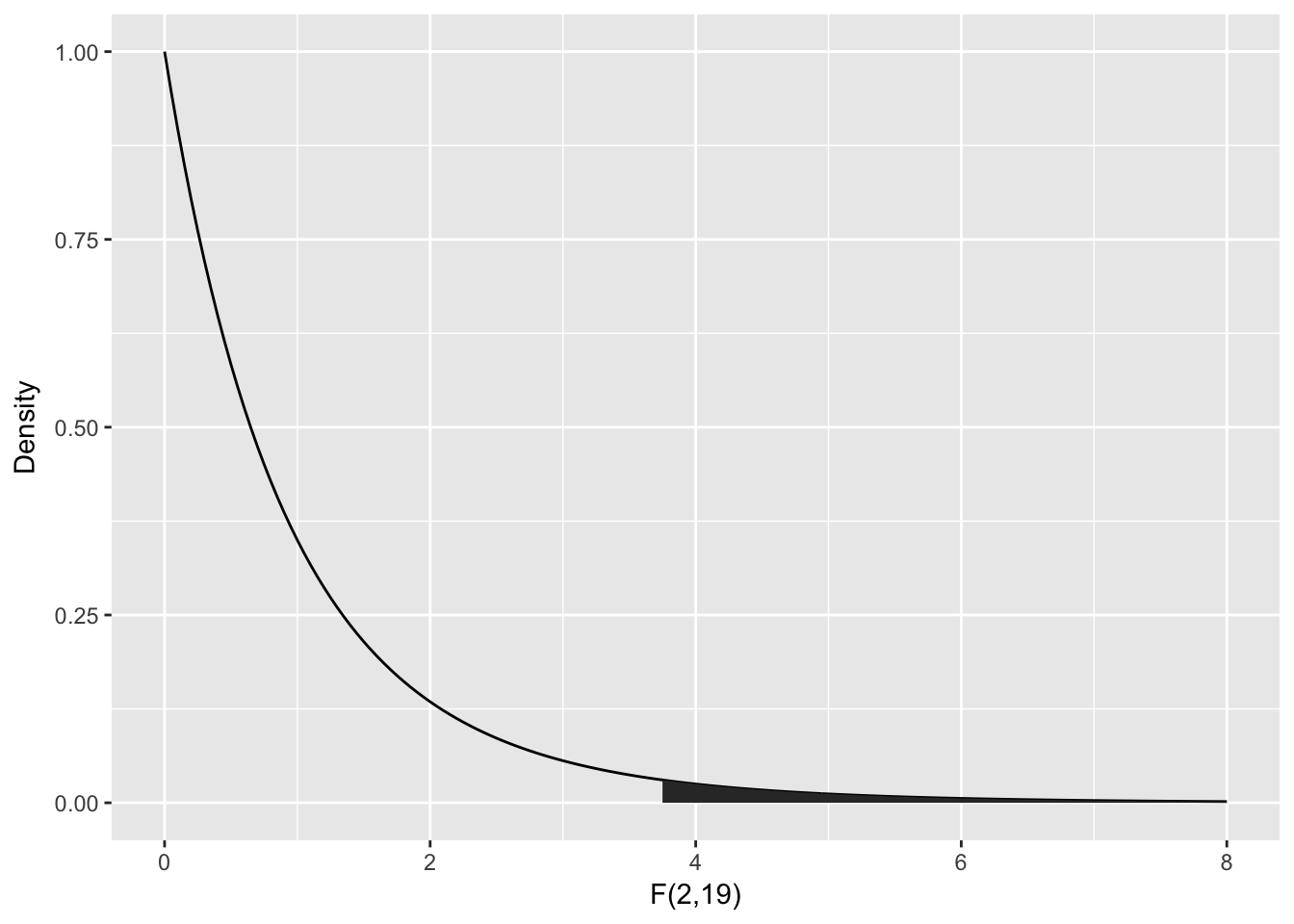
The ANOVA table gives the \(p\)-value as Pr(>F), here \(P = 0.04359\). We could compute this from \(F\) using:
pf(3.7113, df1 = 2, df2 = 19, lower.tail = FALSE)## [1] 0.04359046According to the \(p\)-value, we would reject at the \(\alpha = .05\) level, but some caution is in order.
Let’s continue by checking the assumptions in the model. As in regression, plotting the linear model object results in a series of residual plots.
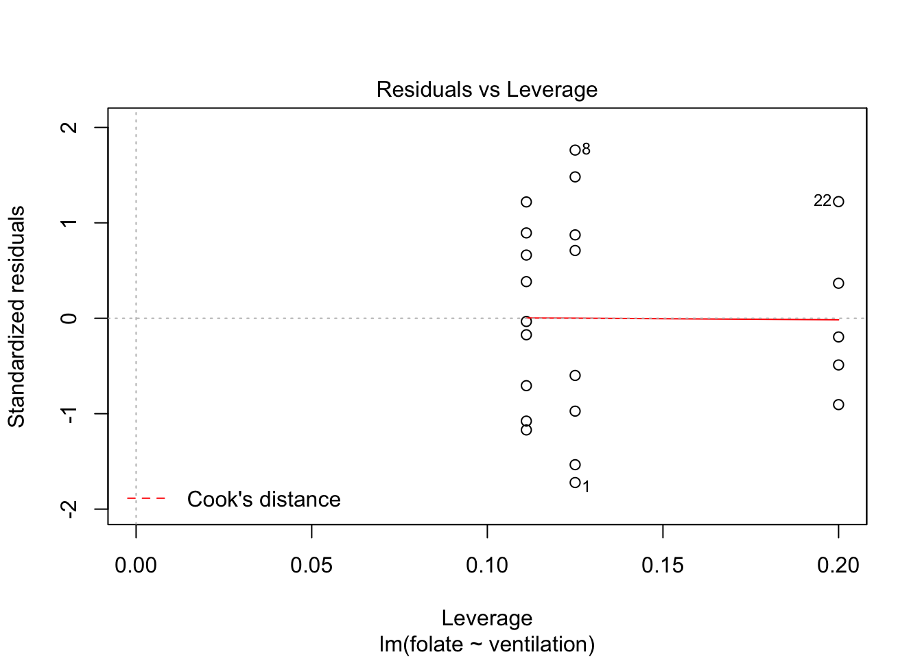
plot(rcf.mod)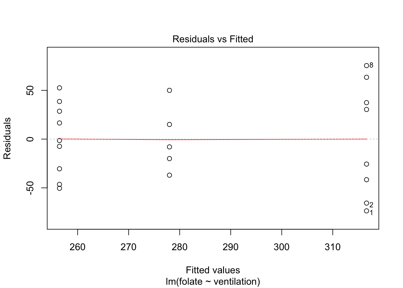
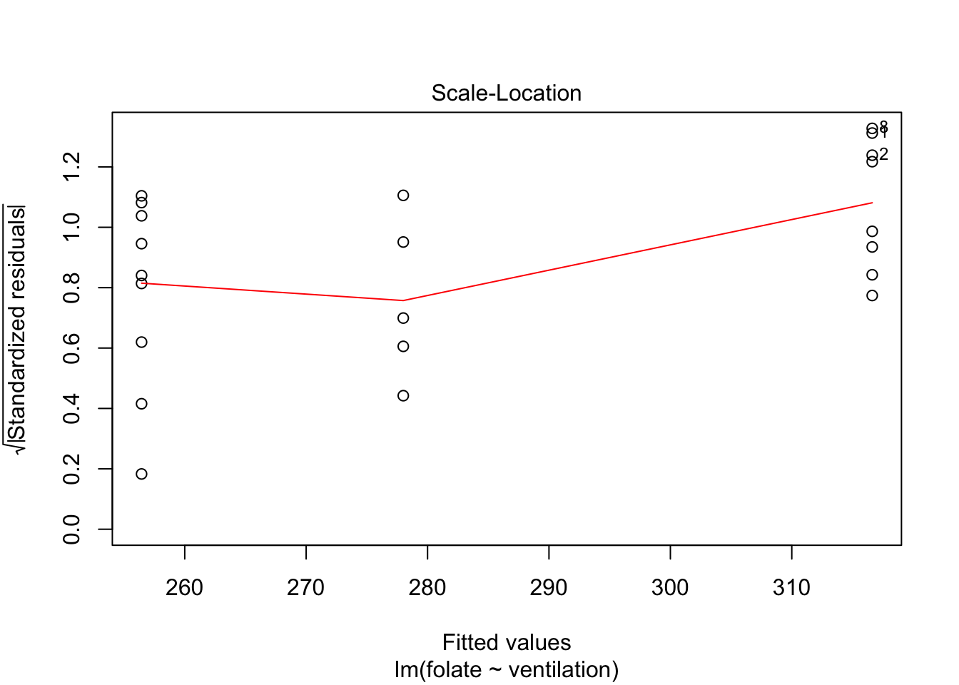
The variances of each group did not look equal in the boxplot, and the Scale-Location plot suggests that the rightmost group does have somewhat higher variation than the others. The x-axis of these plots show Fitted values, which in ANOVA are the group means. So the rightmost cluster of points corresponds to the group with mean 316, which is group 1, the N2O+O2,24h group.
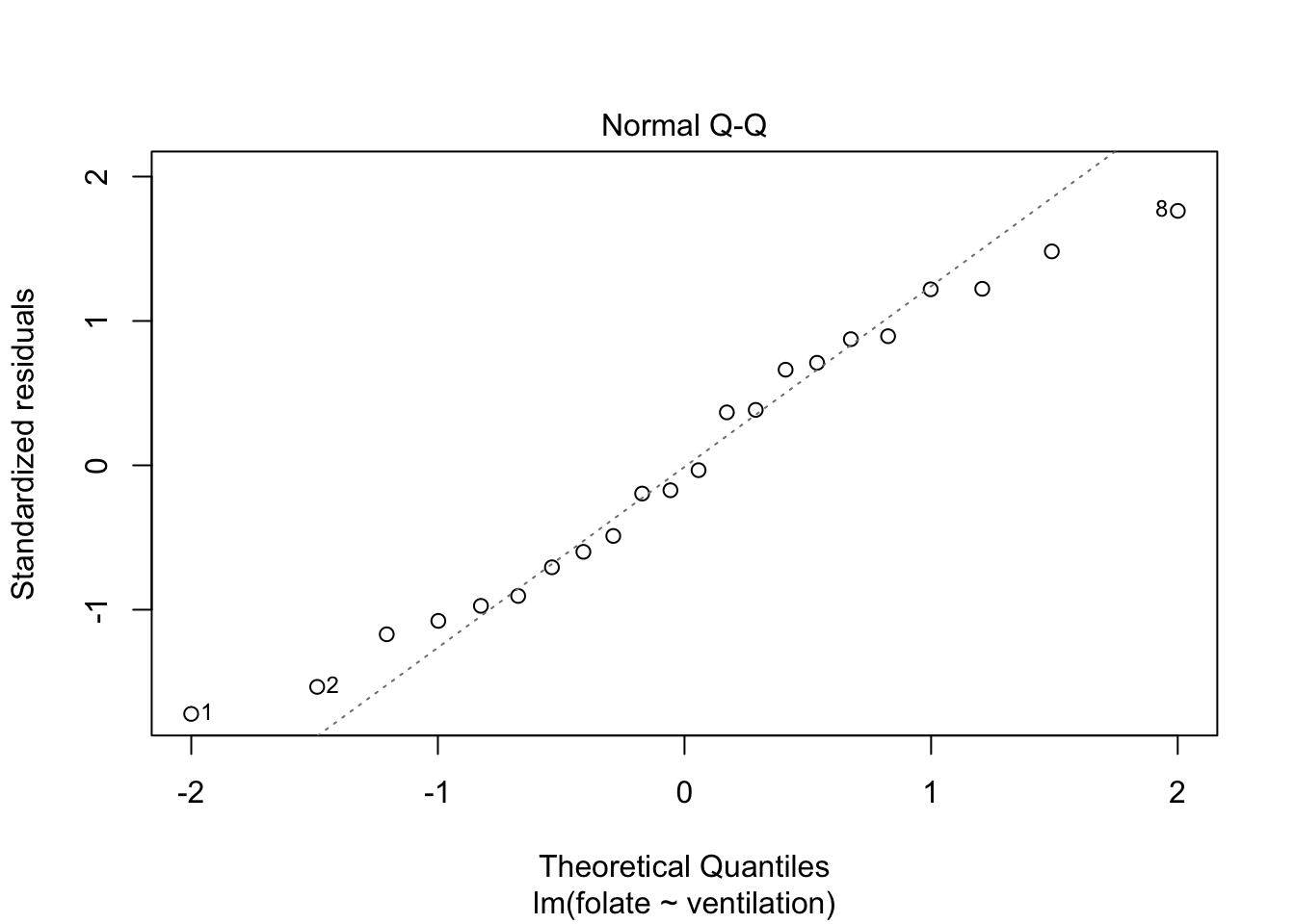
The Normal Q-Q plot suggests the data may be thick tailed. I would put a strongly worded caveat in any report claiming significance based on this data, but it is certainly evidence that perhaps a larger study would be useful.
11.3.2 InsectSprays
The built in data set InsectSprays records the counts of insects in agricultural experimental units treated with different insecticides.
Plotting the data reveals an obvious difference in effectiveness among the spray types:
ggplot(InsectSprays, aes(x=spray, y=count))+geom_boxplot()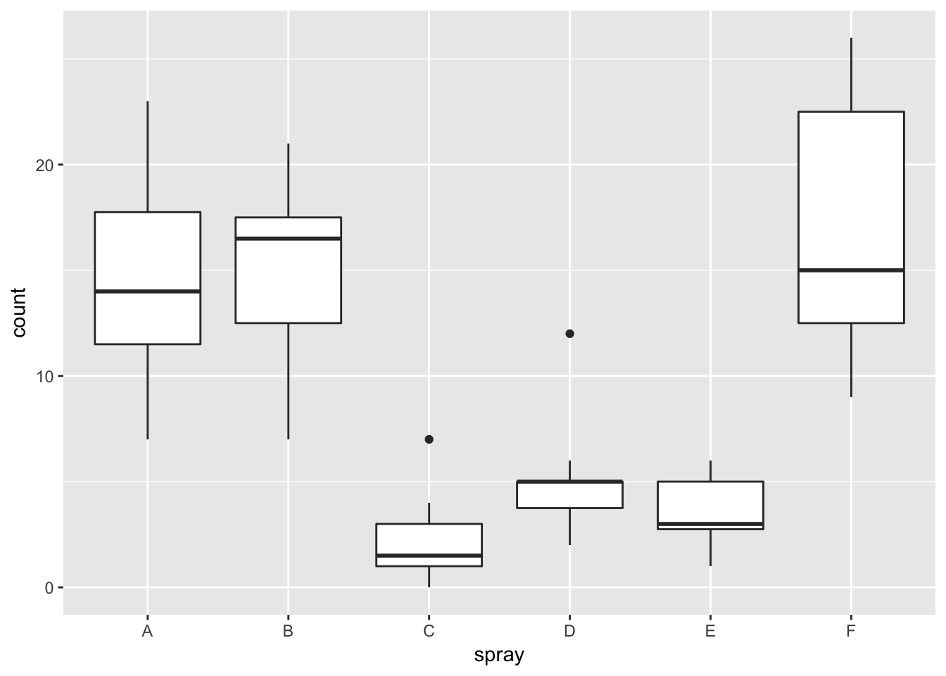
Not surprisingly, ANOVA strongly rejects the null hypothesis that all sprays have the same mean, with a \(p\)-value less than \(2.2 \times 10^{-16}\):
IS.mod <- lm(count ~ spray, data = InsectSprays)
anova(IS.mod)
## Analysis of Variance Table
##
## Response: count
## Df Sum Sq Mean Sq F value Pr(>F)
## spray 5 2668.8 533.77 34.702 < 2.2e-16 ***
## Residuals 66 1015.2 15.38
## ---
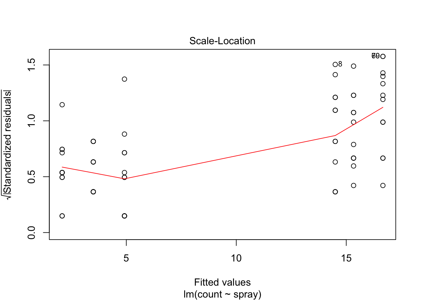
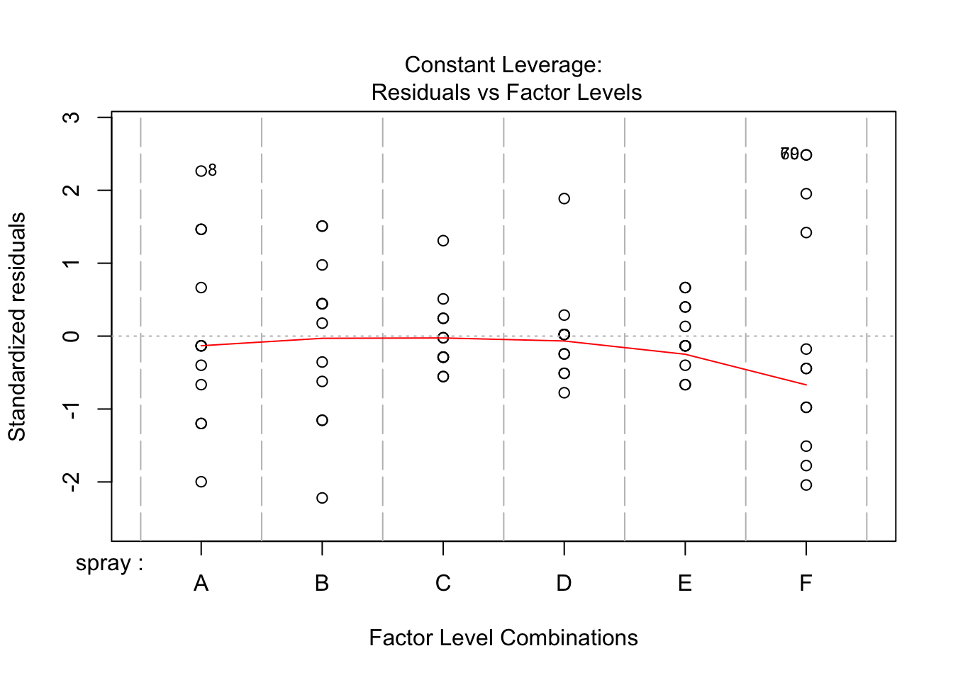
## Signif. codes: 0 '***' 0.001 '**' 0.01 '*' 0.05 '.' 0.1 ' ' 1However, it is also clear from the boxplot that the assumption of equal variances is violated. The three effective sprays C, D, and E, have visibly less variance than the other three sprays. In this example, the sprays with smaller counts have smaller variance. This phenomenon is known as heteroskedacity, and is fairly common. The residual plots show it well, especially the Scale-Location plot
plot(IS.mod)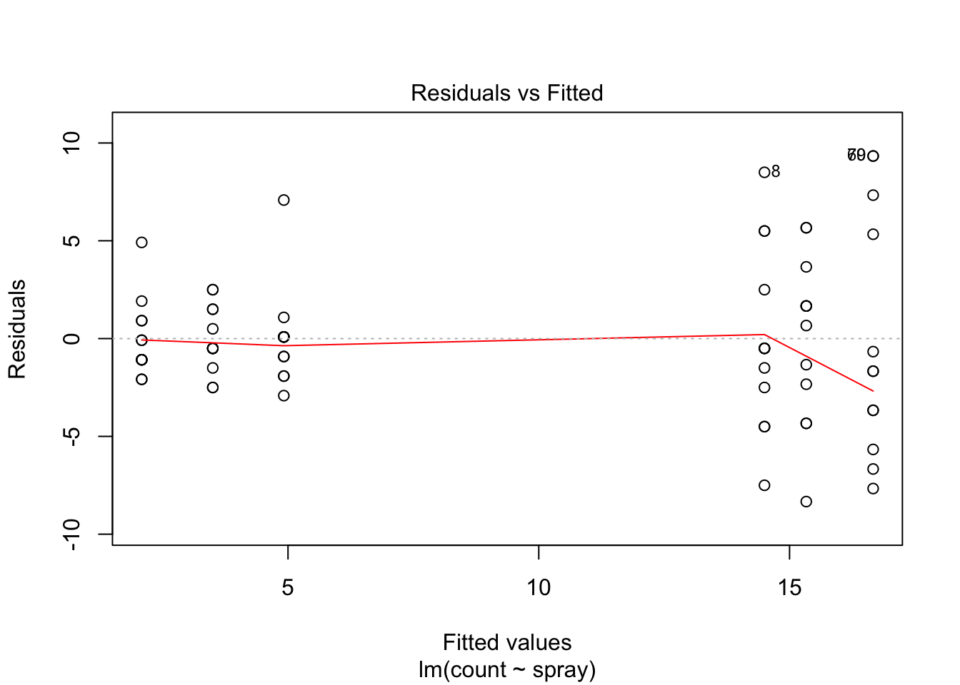
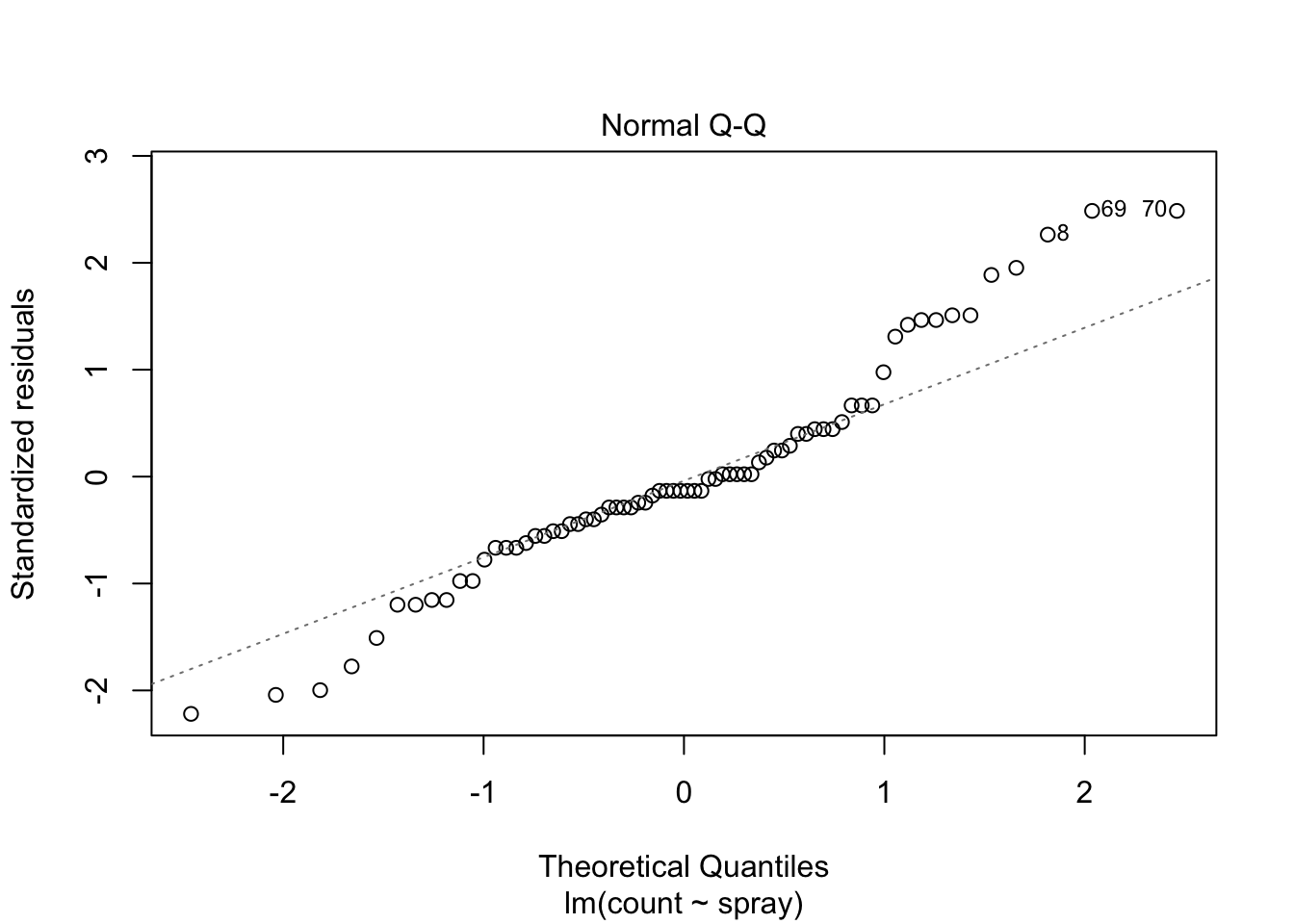
Using ANOVA with this data is highly suspect. Taking the square root of the counts improves the situation, or if normality of the data is not in question, then oneway.test can be used.
ggplot(InsectSprays, aes(x = spray, y = sqrt(count))) + geom_boxplot()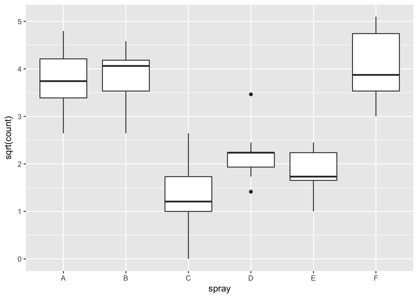
IS.mod <- lm(sqrt(count) ~ spray, data = InsectSprays)
plot(IS.mod)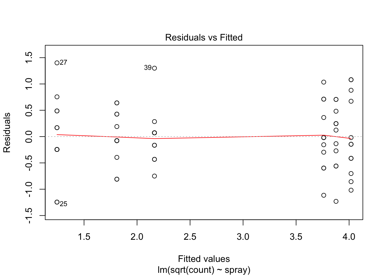
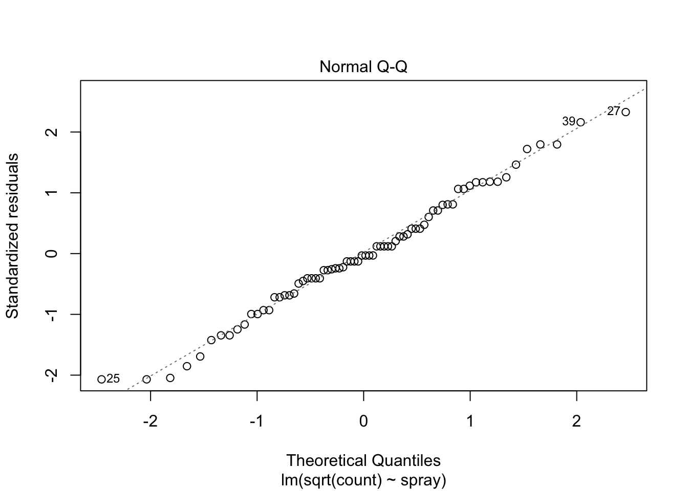
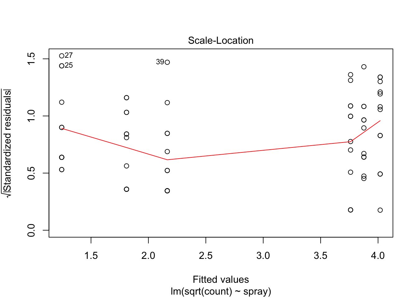
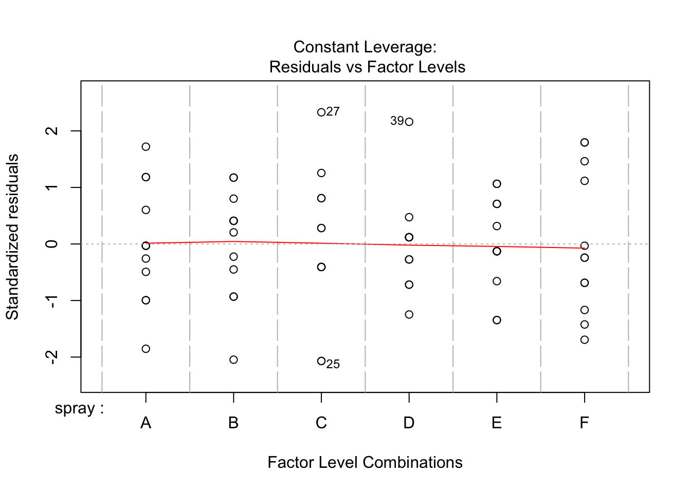
anova(IS.mod)## Analysis of Variance Table
##
## Response: sqrt(count)
## Df Sum Sq Mean Sq F value Pr(>F)
## spray 5 88.438 17.6876 44.799 < 2.2e-16 ***
## Residuals 66 26.058 0.3948
## ---
## Signif. codes: 0 '***' 0.001 '**' 0.01 '*' 0.05 '.' 0.1 ' ' 1Or, if normality of the data within each group is not in question (only the equal variance assumption) then oneway.test can be used.
oneway.test(count~spray, data = InsectSprays)##
## One-way analysis of means (not assuming equal variances)
##
## data: count and spray
## F = 36.065, num df = 5.000, denom df = 30.043, p-value = 7.999e-1211.4 Pairwise t-tests
Suppose we have \(k\) groups of observations. Another approach is to do \({k}\choose{2}\) t-tests, and adjust the \(p\)-values for the fact that we are doing multiple t-tests. This has the advantage of showing directly which pairs of groups have significant differences in means, but the disadvantage of not testing directly \(H_0: \mu_1 = \mu_2 = \cdots = \mu_k\) versus \(H_a:\) at least one of the means is different. See Exercise 6.
For example, returning to the red.cell.folate data, we could do a pairwise t test via the following command:
pairwise.t.test(red.cell.folate$folate, red.cell.folate$ventilation)##
## Pairwise comparisons using t tests with pooled SD
##
## data: red.cell.folate$folate and red.cell.folate$ventilation
##
## N2O+O2,24h N2O+O2,op
## N2O+O2,op 0.042 -
## O2,24h 0.310 0.408
##
## P value adjustment method: holmWe see that there is a significant difference between two of the groups, but not between any of the other pairs. There are several options available with pairwise.t.test, which we discuss below:
pool.sd = TRUEcan be used when we are assuming equal variances among the groups, and we want to use all of the groups together to estimate the standard deviation. This can be useful if one of the groups is small, for example, but it does require the assumption that the variances of each group is the same.p.adjust.methodcan be set to one of several options, which can be viewed by typingp.adjust.methods. The easiest to understand is “bonferroni”, which multiplies the \(p\)-values by the number of tests being performed. This is a very conservative adjustment method! The defaultholmis a good choice. If you wish to compare the results tot.testfor diagnostic purposes, then setp.adust.method = "none".alternative = "greater"or “less” can be used for one sided-tests. Care must be taken to get the order of the groupings correct in this case.var.equal = TRUEcan be used if we know the variances are equal, but we do not want to pool the standard deviation. The default isvar.equal = FALSE, just like int.test. This option is not generally recommended.
11.5 Exercises
- Consider the
case0502data fromSleuth3. Dr Benjamin Spock was tried in Boston for encouraging young men not to register for the draft. It was conjectured that the judge in Spock’s trial did not have appropriate representation of women. The jurors were supposed to be selected by taking a random sample of 30 people (called venires), from which the jurors would be chosen. In the datacase0502, the percent of women in 7 judges’ venires are given.- Create a boxplot of the percent women for each of the 7 judges. Comment on whether you believe that Spock’s lawyers might have a point.
- Determine whether there is a significant difference in the percent of women included in the 6 judges’ venires who aren’t Spock’s judge.
- Determine whether there is a significant difference in the percent of women induced in Spock’s venires versus the percent included in the other judges’ venires combined. (Your answer to a. should justify doing this.)
Consider the data in
ex0524inSleuth3. This gives 2584 data points, where the subjects’ IQ was measured in 1979 and their Income was measured in 2005. Create a boxplot of income for each of the IQ quartiles. Is there evidence to suggest that there is a difference in mean income among the 4 groups of IQ? Check the residuals in your model. Does this cause you to doubt your result?- The built in data set
InsectSpraysrecords the counts of insects in agricultural experimental units treated with different insecticides.- Plot the data. Three of the sprays seem to be more effective (less insects collected) than the other three sprays. Which three are the more effective sprays?
- Use ANOVA to test if the three effective sprays have the same mean. What do you conclude?
- Use ANOVA to test if the three less effective sprays have the same mean. What do you conclude?
The built in data set
chickwtsmeasures weights of chicks after six weeks eating various types of feed. Test if the the mean weight is the same for all feed types. Check the residuals - are the assumptions for ANOVA reasonable?The data set
MASS::immerfrom theMASSlibrary has data on a trial of barley varieties performed by Immer, Hayes, and Powers in the early 1930’s. Test if the total yield (sum of 1931 and 1932) depends on the variety of barley. Check the residuals - are the assumptions for ANOVA reasonable?- Suppose you have 6 groups of 15 observations each. Groups 1-3 are normal with mean 0 and standard deviation 3, while groups 4-6 are normal with mean 1 and standard deviation 3. Compare via simulation the power of the following tests of \(H_0: \mu_1 = \cdot = \mu_6\) versus the alternative that at least one pair is different at the \(\alpha = .05\) level.
- ANOVA. (Hint:
anova(lm(formula, data))[1,5]pulls out the p-value of ANOVA.) - pairwise.t.test, where we reject the null hypothesis if any of the paired \(p\)-values are less than 0.05.
- ANOVA. (Hint: