12 Multiple Regression
In this short chapter, we present an example of linear regression with multiple explanatory variables.
12.0.1 Example One: cystifbr
Consider the data in cystfibr in the library ISwR. Our treatment of this data set follows the treatment given in Dalgaard’s book. Suppose we wish to model the lung capacity in terms of the other variables, based on this data. Let’s get a start by plotting pemax (the measure of lung capacity) versus all of the other variables:
cystfibr <- ISwR::cystfibr
longCyst <- gather(cystfibr, key = variable, value   = value, -pemax)
ggplot(longCyst, aes(x = value, y = pemax)) + geom_point() +
facet_wrap(facets = ~variable, scales = "free_x") 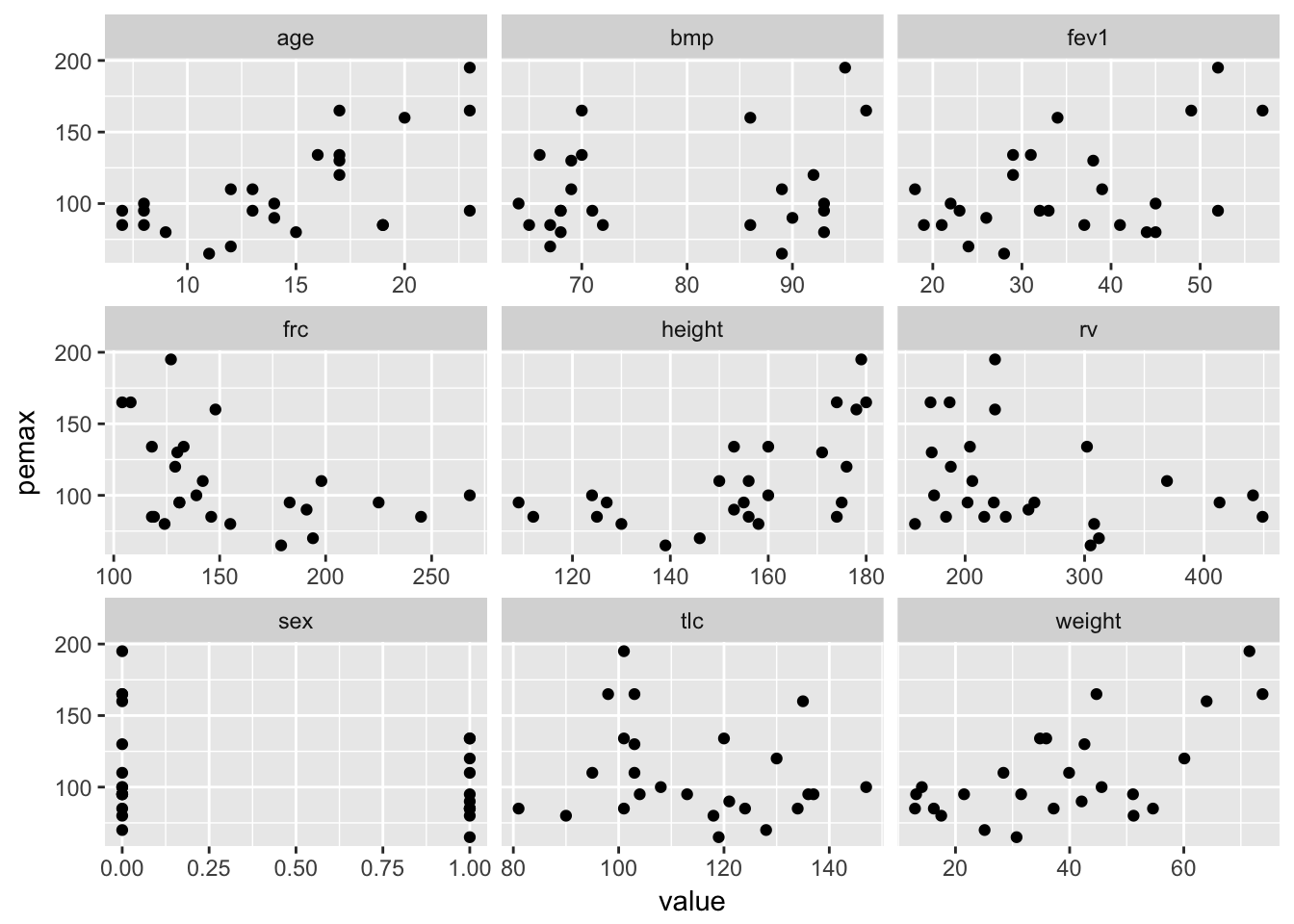
At a first glance, pemax seems correlated with age, weight and height. These variables are also probably strongly correlated with one another, since this is data dealing with adolescents. Let’s check:
cor(cystfibr$age, cystfibr$weight)## [1] 0.9058675cor(cystfibr$age, cystfibr$height)## [1] 0.926052cor(cystfibr$height, cystfibr$weight)## [1] 0.9206953So, yes, they are highly correlated. We are going to run multiple regression on all of the variables at once, and see what we get:
my.mod <- lm(pemax~., data = cystfibr)
summary(my.mod)
##
## Call:
## lm(formula = pemax ~ ., data = cystfibr)
##
## Residuals:
## Min 1Q Median 3Q Max
## -37.338 -11.532 1.081 13.386 33.405
##
## Coefficients:
## Estimate Std. Error t value Pr(>|t|)
## (Intercept) 176.0582 225.8912 0.779 0.448
## age -2.5420 4.8017 -0.529 0.604
## sex -3.7368 15.4598 -0.242 0.812
## height -0.4463 0.9034 -0.494 0.628
## weight 2.9928 2.0080 1.490 0.157
## bmp -1.7449 1.1552 -1.510 0.152
## fev1 1.0807 1.0809 1.000 0.333
## rv 0.1970 0.1962 1.004 0.331
## frc -0.3084 0.4924 -0.626 0.540
## tlc 0.1886 0.4997 0.377 0.711
##
## Residual standard error: 25.47 on 15 degrees of freedom
## Multiple R-squared: 0.6373, Adjusted R-squared: 0.4197
## F-statistic: 2.929 on 9 and 15 DF, p-value: 0.03195A couple of things to notice: first, the p-value is 0.03195, which indicates that the variables together do have a statistically significant predictive value for pemax. However, looking at the list, no one variable seems necessary. The reason for this is that the p-values for each variable is testing what happens when we remove only that variable. So, for example, we can remove weight and not upset the model too much. Of course, since height is strongly correlated with weight, it may just be that height will serve as a proxy for weight in the event that weight is removed!
Let’s look at an anova table:
anova(my.mod)## Analysis of Variance Table
##
## Response: pemax
## Df Sum Sq Mean Sq F value Pr(>F)
## age 1 10098.5 10098.5 15.5661 0.001296 **
## sex 1 955.4 955.4 1.4727 0.243680
## height 1 155.0 155.0 0.2389 0.632089
## weight 1 632.3 632.3 0.9747 0.339170
## bmp 1 2862.2 2862.2 4.4119 0.053010 .
## fev1 1 1549.1 1549.1 2.3878 0.143120
## rv 1 561.9 561.9 0.8662 0.366757
## frc 1 194.6 194.6 0.2999 0.592007
## tlc 1 92.4 92.4 0.1424 0.711160
## Residuals 15 9731.2 648.7
## ---
## Signif. codes: 0 '***' 0.001 '**' 0.01 '*' 0.05 '.' 0.1 ' ' 1We get a different result, because in this case, the table is telling us the significance of adding/removing variables one at a time. For example, age is significant all by itself. Once age is added, sex, height, etc. are not significant. Note that bmp is close to significant. However, we are testing 9 things, so we should expect that relatively often we will get a false small p-value.
One way to test this further is to see whether it is permissible to remove all of the variables once age is included. We do that using anova again.
my.mod2 <- lm(pemax~age, data = cystfibr)
anova(my.mod2, my.mod) #Only use when models are nested! R doesn't check
## Analysis of Variance Table
##
## Model 1: pemax ~ age
## Model 2: pemax ~ age + sex + height + weight + bmp + fev1 + rv + frc +
## tlc
## Res.Df RSS Df Sum of Sq F Pr(>F)
## 1 23 16734.2
## 2 15 9731.2 8 7002.9 1.3493 0.2936As you can see, the p-value is 0.2936, which is not significant. Therefore, we can reasonably conclude that once age is included in the model, that is about as good as we can do. Note: This does NOT mean that age is necessarily the best predictor of pemax. The reason that it was included in the final model is largely due to the fact that it was listed first in the data set!
Let’s see what happens if we change the order:
my.mod <- lm(pemax~height+age+weight+sex+bmp+fev1+rv+frc+tlc, data = cystfibr)
summary(my.mod)
##
## Call:
## lm(formula = pemax ~ height + age + weight + sex + bmp + fev1 +
## rv + frc + tlc, data = cystfibr)
##
## Residuals:
## Min 1Q Median 3Q Max
## -37.338 -11.532 1.081 13.386 33.405
##
## Coefficients:
## Estimate Std. Error t value Pr(>|t|)
## (Intercept) 176.0582 225.8912 0.779 0.448
## height -0.4463 0.9034 -0.494 0.628
## age -2.5420 4.8017 -0.529 0.604
## weight 2.9928 2.0080 1.490 0.157
## sex -3.7368 15.4598 -0.242 0.812
## bmp -1.7449 1.1552 -1.510 0.152
## fev1 1.0807 1.0809 1.000 0.333
## rv 0.1970 0.1962 1.004 0.331
## frc -0.3084 0.4924 -0.626 0.540
## tlc 0.1886 0.4997 0.377 0.711
##
## Residual standard error: 25.47 on 15 degrees of freedom
## Multiple R-squared: 0.6373, Adjusted R-squared: 0.4197
## F-statistic: 2.929 on 9 and 15 DF, p-value: 0.03195Note that the overall p-value is the same.
anova(my.mod)## Analysis of Variance Table
##
## Response: pemax
## Df Sum Sq Mean Sq F value Pr(>F)
## height 1 9634.6 9634.6 14.8511 0.001562 **
## age 1 646.2 646.2 0.9960 0.334098
## weight 1 769.6 769.6 1.1863 0.293271
## sex 1 790.8 790.8 1.2189 0.286964
## bmp 1 2862.2 2862.2 4.4119 0.053010 .
## fev1 1 1549.1 1549.1 2.3878 0.143120
## rv 1 561.9 561.9 0.8662 0.366757
## frc 1 194.6 194.6 0.2999 0.592007
## tlc 1 92.4 92.4 0.1424 0.711160
## Residuals 15 9731.2 648.7
## ---
## Signif. codes: 0 '***' 0.001 '**' 0.01 '*' 0.05 '.' 0.1 ' ' 1Here, we see that height is significant, and nothing else. If we test the model pemax ~ height versus pemax ~ ., we get
anova(my.mod2, my.mod) #Only use when models are nested!## Analysis of Variance Table
##
## Model 1: pemax ~ age
## Model 2: pemax ~ height + age + weight + sex + bmp + fev1 + rv + frc +
## tlc
## Res.Df RSS Df Sum of Sq F Pr(>F)
## 1 23 16734.2
## 2 15 9731.2 8 7002.9 1.3493 0.2936And again, we can conclude that once we have added height, there is not much to be gained by adding other variables. We leave it to the reader to test whether weight follows the same pattern as height and age.
Let’s first examine a couple of other ways we could have proceeded.
my.mod <- lm(pemax~., data = cystfibr)
summary(my.mod)
##
## Call:
## lm(formula = pemax ~ ., data = cystfibr)
##
## Residuals:
## Min 1Q Median 3Q Max
## -37.338 -11.532 1.081 13.386 33.405
##
## Coefficients:
## Estimate Std. Error t value Pr(>|t|)
## (Intercept) 176.0582 225.8912 0.779 0.448
## age -2.5420 4.8017 -0.529 0.604
## sex -3.7368 15.4598 -0.242 0.812
## height -0.4463 0.9034 -0.494 0.628
## weight 2.9928 2.0080 1.490 0.157
## bmp -1.7449 1.1552 -1.510 0.152
## fev1 1.0807 1.0809 1.000 0.333
## rv 0.1970 0.1962 1.004 0.331
## frc -0.3084 0.4924 -0.626 0.540
## tlc 0.1886 0.4997 0.377 0.711
##
## Residual standard error: 25.47 on 15 degrees of freedom
## Multiple R-squared: 0.6373, Adjusted R-squared: 0.4197
## F-statistic: 2.929 on 9 and 15 DF, p-value: 0.03195We start to eliminate variables that are not statistically significant in the model. We will begin with the other lung function data, for as long as we are allowed to continue to remove. The order chosen for removal is: tlc, frc, rv, fev1.
summary(lm(pemax~height+age+weight+sex+bmp+fev1+rv+frc, data = cystfibr))##
## Call:
## lm(formula = pemax ~ height + age + weight + sex + bmp + fev1 +
## rv + frc, data = cystfibr)
##
## Residuals:
## Min 1Q Median 3Q Max
## -38.072 -10.067 0.113 13.526 36.990
##
## Coefficients:
## Estimate Std. Error t value Pr(>|t|)
## (Intercept) 221.8055 185.4350 1.196 0.2491
## height -0.5428 0.8428 -0.644 0.5286
## age -3.1346 4.4144 -0.710 0.4879
## weight 3.3157 1.7672 1.876 0.0790 .
## sex -4.6933 14.8363 -0.316 0.7558
## bmp -1.9403 1.0047 -1.931 0.0714 .
## fev1 1.0183 1.0392 0.980 0.3417
## rv 0.1857 0.1887 0.984 0.3396
## frc -0.2605 0.4628 -0.563 0.5813
## ---
## Signif. codes: 0 '***' 0.001 '**' 0.01 '*' 0.05 '.' 0.1 ' ' 1
##
## Residual standard error: 24.78 on 16 degrees of freedom
## Multiple R-squared: 0.6339, Adjusted R-squared: 0.4508
## F-statistic: 3.463 on 8 and 16 DF, p-value: 0.01649summary(lm(pemax~height+age+weight+sex+bmp+fev1+rv, data = cystfibr))##
## Call:
## lm(formula = pemax ~ height + age + weight + sex + bmp + fev1 +
## rv, data = cystfibr)
##
## Residuals:
## Min 1Q Median 3Q Max
## -39.425 -12.391 3.834 14.797 36.693
##
## Coefficients:
## Estimate Std. Error t value Pr(>|t|)
## (Intercept) 166.71822 154.31294 1.080 0.2951
## height -0.40981 0.79257 -0.517 0.6118
## age -1.81783 3.66773 -0.496 0.6265
## weight 2.87386 1.55120 1.853 0.0814 .
## sex 0.10239 11.89990 0.009 0.9932
## bmp -1.94971 0.98415 -1.981 0.0640 .
## fev1 1.41526 0.74788 1.892 0.0756 .
## rv 0.09567 0.09798 0.976 0.3425
## ---
## Signif. codes: 0 '***' 0.001 '**' 0.01 '*' 0.05 '.' 0.1 ' ' 1
##
## Residual standard error: 24.28 on 17 degrees of freedom
## Multiple R-squared: 0.6266, Adjusted R-squared: 0.4729
## F-statistic: 4.076 on 7 and 17 DF, p-value: 0.008452summary(lm(pemax~height+age+weight+sex+bmp+fev1, data = cystfibr))##
## Call:
## lm(formula = pemax ~ height + age + weight + sex + bmp + fev1,
## data = cystfibr)
##
## Residuals:
## Min 1Q Median 3Q Max
## -43.238 -7.403 -0.081 15.534 36.028
##
## Coefficients:
## Estimate Std. Error t value Pr(>|t|)
## (Intercept) 260.6313 120.5215 2.163 0.0443 *
## height -0.6067 0.7655 -0.793 0.4384
## age -2.9062 3.4898 -0.833 0.4159
## weight 3.3463 1.4719 2.273 0.0355 *
## sex -1.2115 11.8083 -0.103 0.9194
## bmp -2.3042 0.9136 -2.522 0.0213 *
## fev1 1.0274 0.6329 1.623 0.1219
## ---
## Signif. codes: 0 '***' 0.001 '**' 0.01 '*' 0.05 '.' 0.1 ' ' 1
##
## Residual standard error: 24.24 on 18 degrees of freedom
## Multiple R-squared: 0.6057, Adjusted R-squared: 0.4743
## F-statistic: 4.608 on 6 and 18 DF, p-value: 0.00529summary(lm(pemax~height+age+weight+sex+bmp, data = cystfibr))##
## Call:
## lm(formula = pemax ~ height + age + weight + sex + bmp, data = cystfibr)
##
## Residuals:
## Min 1Q Median 3Q Max
## -43.194 -9.412 -2.425 9.157 40.112
##
## Coefficients:
## Estimate Std. Error t value Pr(>|t|)
## (Intercept) 280.4482 124.9556 2.244 0.0369 *
## height -0.6853 0.7962 -0.861 0.4001
## age -3.0750 3.6352 -0.846 0.4081
## weight 3.5546 1.5281 2.326 0.0312 *
## sex -11.5281 10.3720 -1.111 0.2802
## bmp -1.9613 0.9263 -2.117 0.0476 *
## ---
## Signif. codes: 0 '***' 0.001 '**' 0.01 '*' 0.05 '.' 0.1 ' ' 1
##
## Residual standard error: 25.27 on 19 degrees of freedom
## Multiple R-squared: 0.548, Adjusted R-squared: 0.429
## F-statistic: 4.606 on 5 and 19 DF, p-value: 0.006388When removing variables in a stepwise manner such as above, it is important to consider adding variables back into the model. Since we have removed all of the lung function data one variable at a time, let’s see whether the group of lung function data is significant as a whole. This serves as a sort of test as to whether we need to consider adding variables back in to the model.
mod1 <- lm(pemax~., data = cystfibr)
mod2 <- lm(pemax~height+age+weight+sex+bmp, data = cystfibr)
anova(mod2, mod1)
## Analysis of Variance Table
##
## Model 1: pemax ~ height + age + weight + sex + bmp
## Model 2: pemax ~ age + sex + height + weight + bmp + fev1 + rv + frc +
## tlc
## Res.Df RSS Df Sum of Sq F Pr(>F)
## 1 19 12129.2
## 2 15 9731.2 4 2398 0.9241 0.4758Since the \(p\)-value is 0.4758, this is an indication that the group of variables is not significant as a whole, and we are at least somewhat justified in removing the group.
Returning to variable selection, we see that age, height and sex don’t seem important, so let’s start removing.
summary(lm(pemax~height+weight+sex+bmp, data = cystfibr))##
## Call:
## lm(formula = pemax ~ height + weight + sex + bmp, data = cystfibr)
##
## Residuals:
## Min 1Q Median 3Q Max
## -46.202 -11.699 -1.845 10.322 38.744
##
## Coefficients:
## Estimate Std. Error t value Pr(>|t|)
## (Intercept) 251.3973 119.2859 2.108 0.0479 *
## height -0.8128 0.7762 -1.047 0.3075
## weight 2.6947 1.1329 2.379 0.0275 *
## sex -11.5458 10.2979 -1.121 0.2755
## bmp -1.4881 0.7330 -2.030 0.0558 .
## ---
## Signif. codes: 0 '***' 0.001 '**' 0.01 '*' 0.05 '.' 0.1 ' ' 1
##
## Residual standard error: 25.09 on 20 degrees of freedom
## Multiple R-squared: 0.5309, Adjusted R-squared: 0.4371
## F-statistic: 5.66 on 4 and 20 DF, p-value: 0.003253summary(lm(pemax~weight+sex+bmp, data = cystfibr))##
## Call:
## lm(formula = pemax ~ weight + sex + bmp, data = cystfibr)
##
## Residuals:
## Min 1Q Median 3Q Max
## -47.05 -11.65 4.23 13.75 45.35
##
## Coefficients:
## Estimate Std. Error t value Pr(>|t|)
## (Intercept) 132.9306 37.9132 3.506 0.002101 **
## weight 1.5810 0.3910 4.044 0.000585 ***
## sex -11.7140 10.3203 -1.135 0.269147
## bmp -1.0140 0.5777 -1.755 0.093826 .
## ---
## Signif. codes: 0 '***' 0.001 '**' 0.01 '*' 0.05 '.' 0.1 ' ' 1
##
## Residual standard error: 25.14 on 21 degrees of freedom
## Multiple R-squared: 0.5052, Adjusted R-squared: 0.4345
## F-statistic: 7.148 on 3 and 21 DF, p-value: 0.001732summary(lm(pemax~weight+bmp, data = cystfibr))##
## Call:
## lm(formula = pemax ~ weight + bmp, data = cystfibr)
##
## Residuals:
## Min 1Q Median 3Q Max
## -42.924 -13.399 4.361 16.642 48.404
##
## Coefficients:
## Estimate Std. Error t value Pr(>|t|)
## (Intercept) 124.8297 37.4786 3.331 0.003033 **
## weight 1.6403 0.3900 4.206 0.000365 ***
## bmp -1.0054 0.5814 -1.729 0.097797 .
## ---
## Signif. codes: 0 '***' 0.001 '**' 0.01 '*' 0.05 '.' 0.1 ' ' 1
##
## Residual standard error: 25.31 on 22 degrees of freedom
## Multiple R-squared: 0.4749, Adjusted R-squared: 0.4271
## F-statistic: 9.947 on 2 and 22 DF, p-value: 0.0008374Again, we have removed a group of variables that are related, so let’s see if the group as a whole is significant. If it were, then we would need to consider adding variables back in to our model.
mod3 <- lm(pemax~weight+bmp, data = cystfibr)
anova(mod3, mod2)
## Analysis of Variance Table
##
## Model 1: pemax ~ weight + bmp
## Model 2: pemax ~ height + age + weight + sex + bmp
## Res.Df RSS Df Sum of Sq F Pr(>F)
## 1 22 14090
## 2 19 12129 3 1961.3 1.0241 0.4041This indicates that we are justified in removing the age, weight and sex variables. And now, bmp also doesn’t seem important. We are left with modeling pemax on weight, similar to what we had before.
There is a built-in R function that does variable selection using the Akaike Information Content. This is a different criterion than the \(p\)-value criterion that we were using above, and you typically get difference models. Recall that mod1 is the full model.
aicMod <- step(mod1, direction = "both", trace = FALSE)
summary(aicMod)
##
## Call:
## lm(formula = pemax ~ weight + bmp + fev1 + rv, data = cystfibr)
##
## Residuals:
## Min 1Q Median 3Q Max
## -39.77 -11.74 4.33 15.66 35.07
##
## Coefficients:
## Estimate Std. Error t value Pr(>|t|)
## (Intercept) 63.94669 53.27673 1.200 0.244057
## weight 1.74891 0.38063 4.595 0.000175 ***
## bmp -1.37724 0.56534 -2.436 0.024322 *
## fev1 1.54770 0.57761 2.679 0.014410 *
## rv 0.12572 0.08315 1.512 0.146178
## ---
## Signif. codes: 0 '***' 0.001 '**' 0.01 '*' 0.05 '.' 0.1 ' ' 1
##
## Residual standard error: 22.75 on 20 degrees of freedom
## Multiple R-squared: 0.6141, Adjusted R-squared: 0.5369
## F-statistic: 7.957 on 4 and 20 DF, p-value: 0.000523As is typical, the step procedure leaves more variables in the model than our \(p\)-value criterion. In this case, we would mode pemax on weight, bmp, fev1 and rv.
Returning to the model of pemax on height, let’s take a look at the residuals.
my.mod <- lm(pemax~height, data = cystfibr)
plot(pemax~height, data = cystfibr)
abline(my.mod)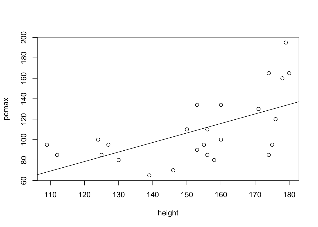
plot(my.mod)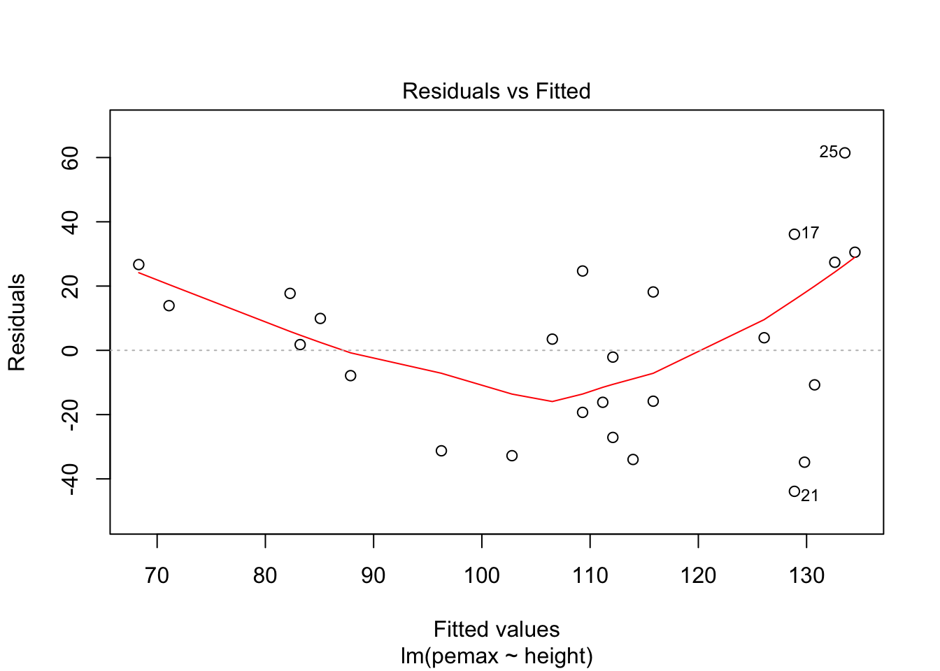
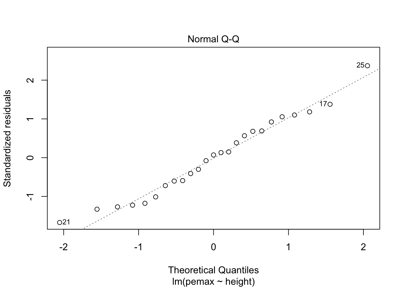
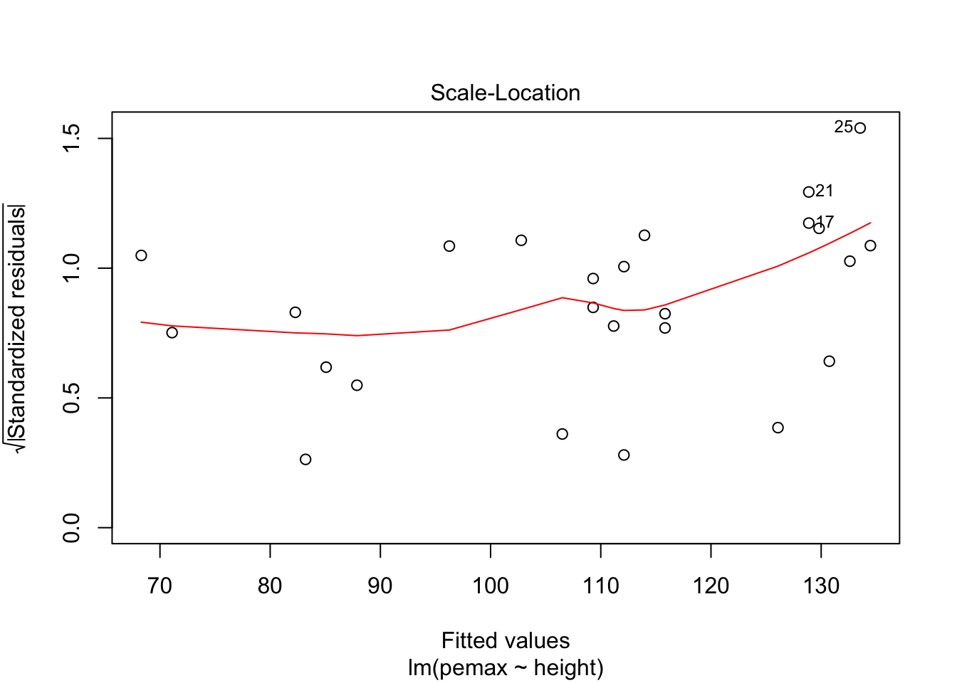
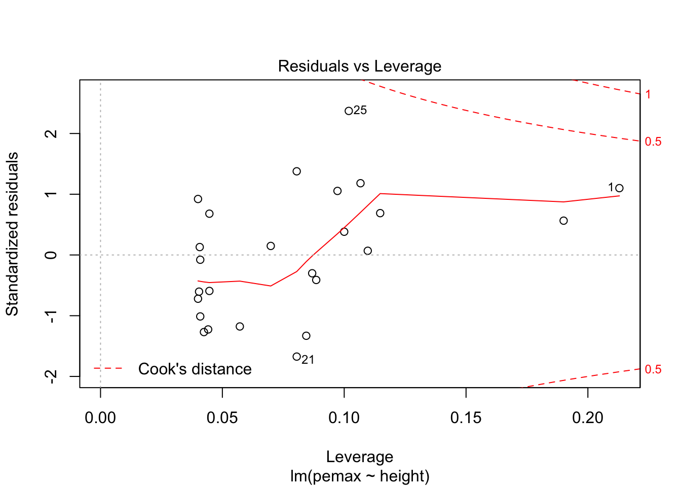
It is hard to say, but there definitely could be a U-shape in the Residuals vs Fitted plot, which means there might be some lurking variables that we have not yet taken into account. One possibility is that pemax actually depends on height and height-sqaured, rather than height itself. Let’s see what happens when we run the model:
my.mod2 <- lm(pemax~height + I(height^2), data = cystfibr)
summary(my.mod2)
##
## Call:
## lm(formula = pemax ~ height + I(height^2), data = cystfibr)
##
## Residuals:
## Min 1Q Median 3Q Max
## -51.411 -14.932 -2.288 12.787 44.933
##
## Coefficients:
## Estimate Std. Error t value Pr(>|t|)
## (Intercept) 615.36248 240.95580 2.554 0.0181 *
## height -8.08324 3.32052 -2.434 0.0235 *
## I(height^2) 0.03064 0.01126 2.721 0.0125 *
## ---
## Signif. codes: 0 '***' 0.001 '**' 0.01 '*' 0.05 '.' 0.1 ' ' 1
##
## Residual standard error: 24.18 on 22 degrees of freedom
## Multiple R-squared: 0.5205, Adjusted R-squared: 0.4769
## F-statistic: 11.94 on 2 and 22 DF, p-value: 0.0003081Notice that in this case, both height and height^2 are significant.
Aside Let’s pause and think a moment about what we are doing. If we assume that we are just exploring the data, then the process that has led us to considering modeling pemax as a function of height and height^2 is marginal. Considering that pemax seems to have larger variance for taller children, it is not hard to imagine that a linear relationship could look quadratic. We also have no a prioiri reason to think that pemax might depend on height^2. So, think of this as an illustration of what can be done and not necessarily an ideal analysis of the data. A couple of things that might be reasonable would be to either (1) contact the experts to see whether there is any reason that height^2 might be relevant, and (2) collect more data and see whether the relationship was an artifact of this data or whether it is recreated the second time around. End of Aside
Let’s check the residuals:
plot(my.mod2)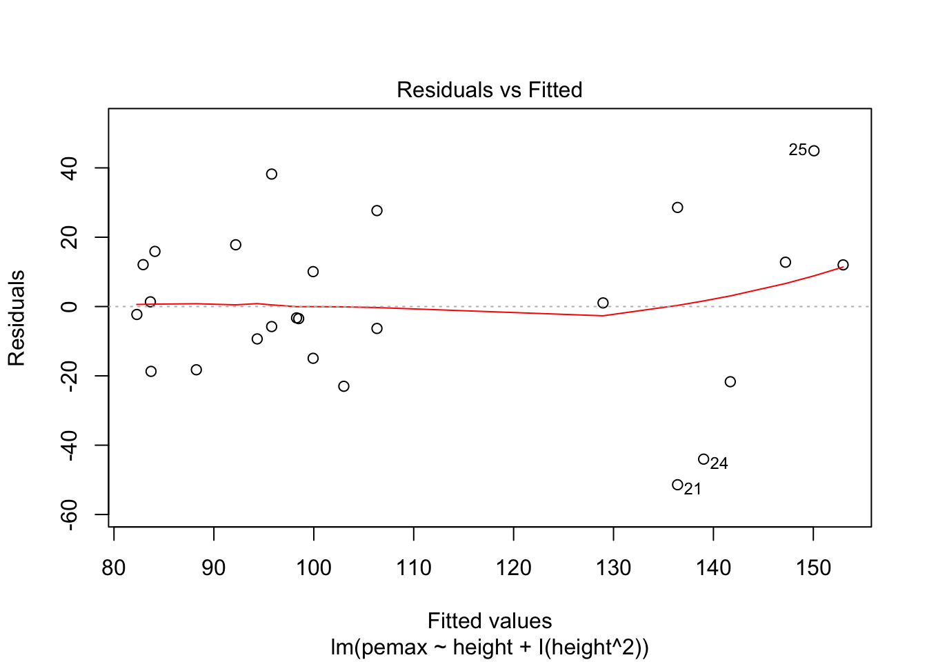
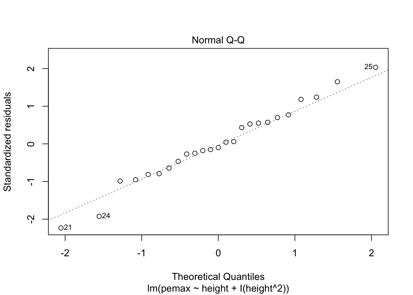
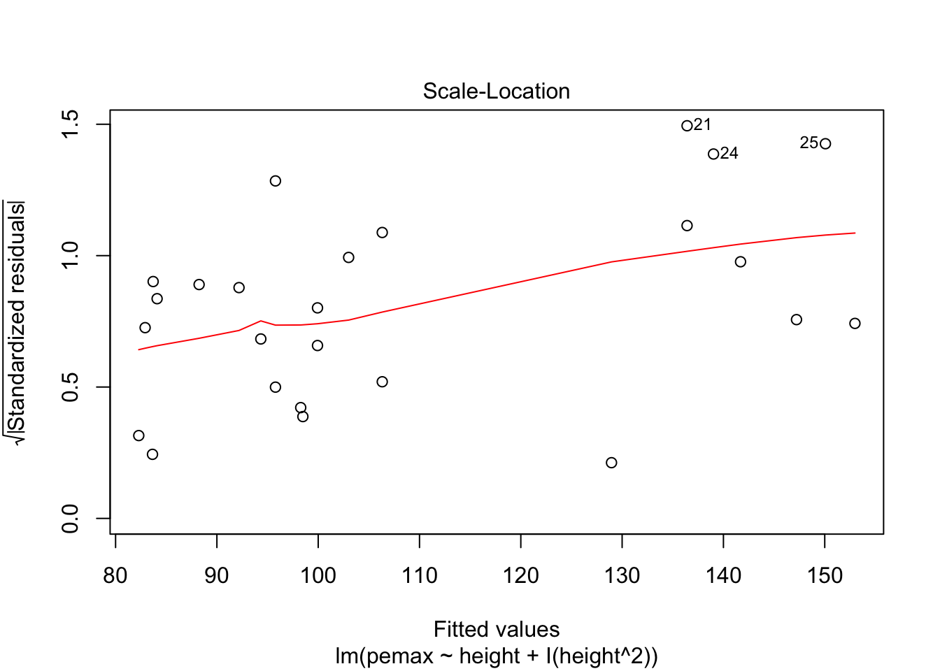
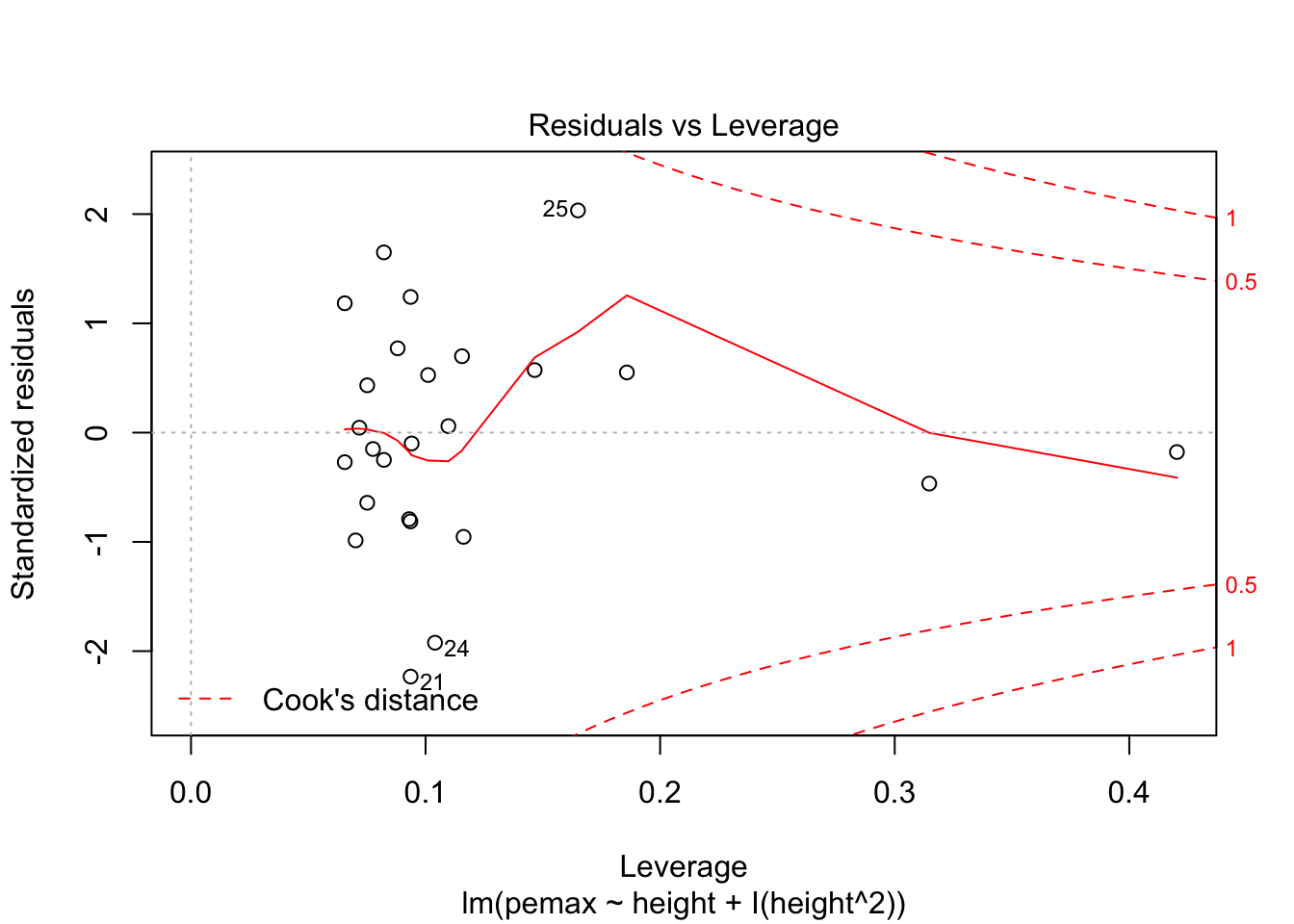
Looks pretty good, except we seem to be violating constant variance. In particular, the variance seems to be higher for children with higher height/pemax values than for shorter children. Let’s re-examine the plot of pemax vs height:
ggplot(cystfibr, aes(x = height, y = pemax)) + geom_point()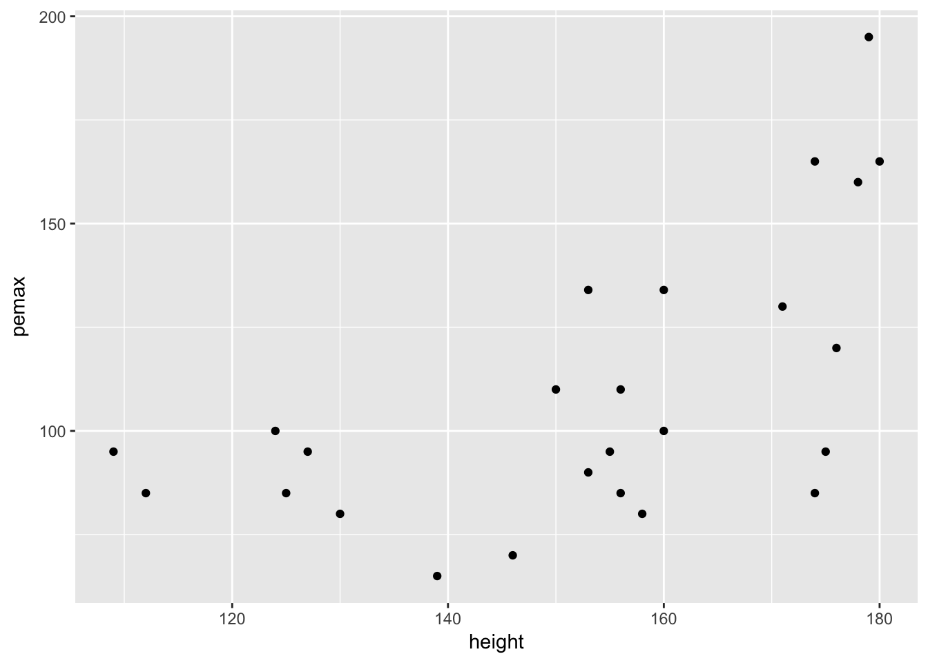
This plot also seems to show that the variance of pemax depends on the height of the child.
12.0.2 Example Two: Secher data
Let’s examine the secher data. Here, we have the birth weight of 107 babies, together with two diameter measurements.
secher <- ISwR::secher
secher$no <- NULL
longSecher <- gather(data = secher, key = variable, value = value, -bwt)
ggplot(longSecher, aes(x = value, y = bwt)) + geom_point() +
  facet_wrap(facets = ~variable, scales = "free_x")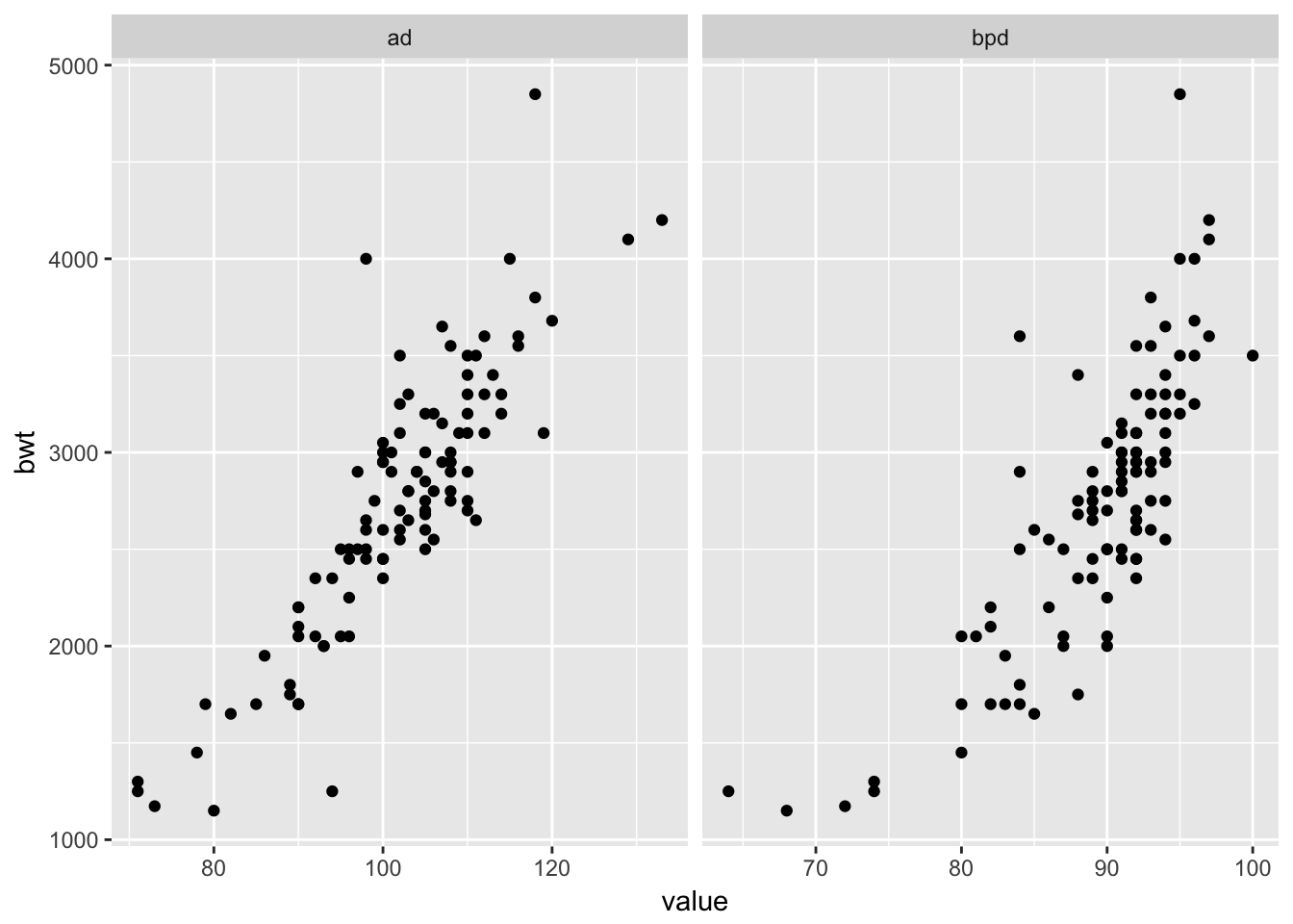
A brief glance at the plots (especially bwt versus bpd) gives an indication that the variance is not constant. Let’s use a log transformation of all three variables, and plot again.
longSecher$value <- log(longSecher$value)
longSecher$bwt <- log(longSecher$bwt)
ggplot(longSecher, aes(x = value, y = bwt)) + geom_point() +
  facet_wrap(facets = ~variable, scales = "free_x")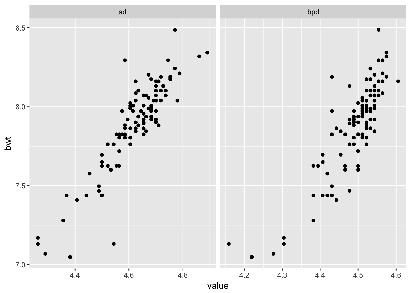
As you can see by the plots, the data seems more linear, and the variance seems to be constant across scales. Now, we model log(bwt) on log of the other two variables.
my.mod <- lm(I(log(bwt))~I(log(bpd)) + I(log(ad)), data = secher)
summary(my.mod)
##
## Call:
## lm(formula = I(log(bwt)) ~ I(log(bpd)) + I(log(ad)), data = secher)
##
## Residuals:
## Min 1Q Median 3Q Max
## -0.35074 -0.06741 -0.00792 0.05750 0.36360
##
## Coefficients:
## Estimate Std. Error t value Pr(>|t|)
## (Intercept) -5.8615 0.6617 -8.859 2.36e-14 ***
## I(log(bpd)) 1.5519 0.2294 6.764 8.09e-10 ***
## I(log(ad)) 1.4667 0.1467 9.998 < 2e-16 ***
## ---
## Signif. codes: 0 '***' 0.001 '**' 0.01 '*' 0.05 '.' 0.1 ' ' 1
##
## Residual standard error: 0.1068 on 104 degrees of freedom
## Multiple R-squared: 0.8583, Adjusted R-squared: 0.8556
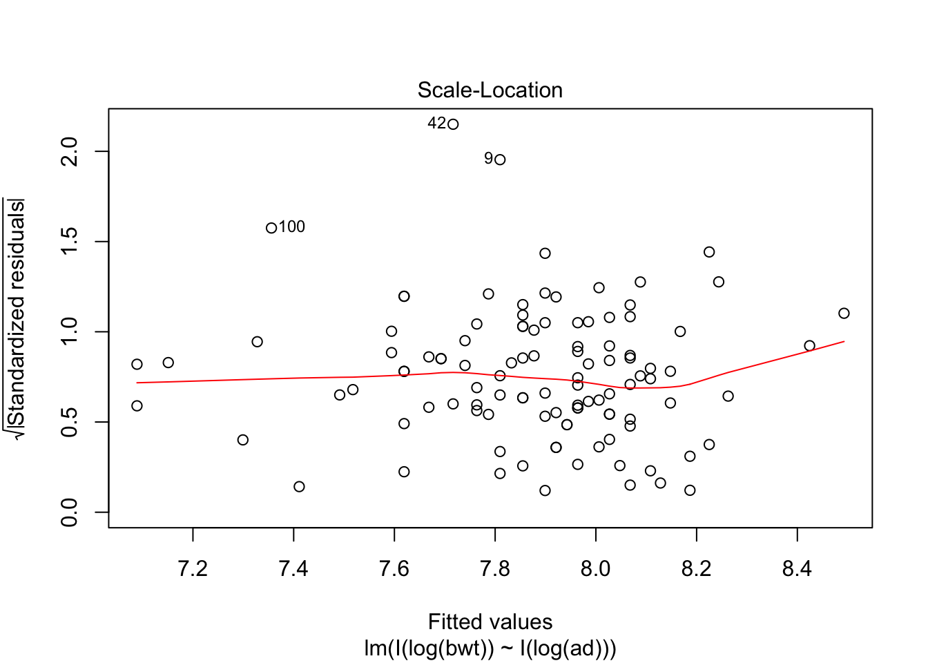
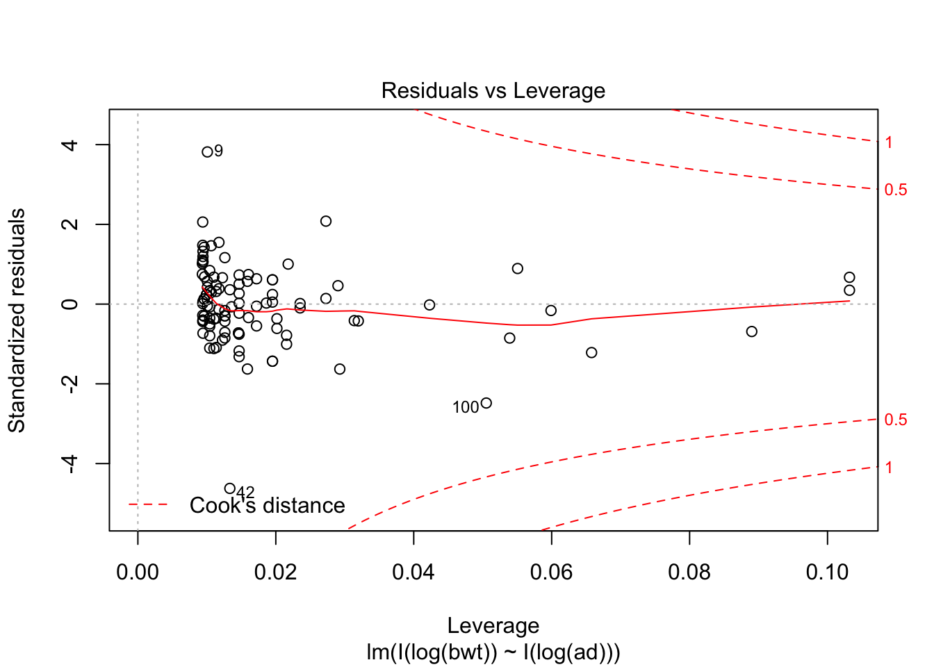
## F-statistic: 314.9 on 2 and 104 DF, p-value: < 2.2e-16plot(my.mod, which = c(1,3,5))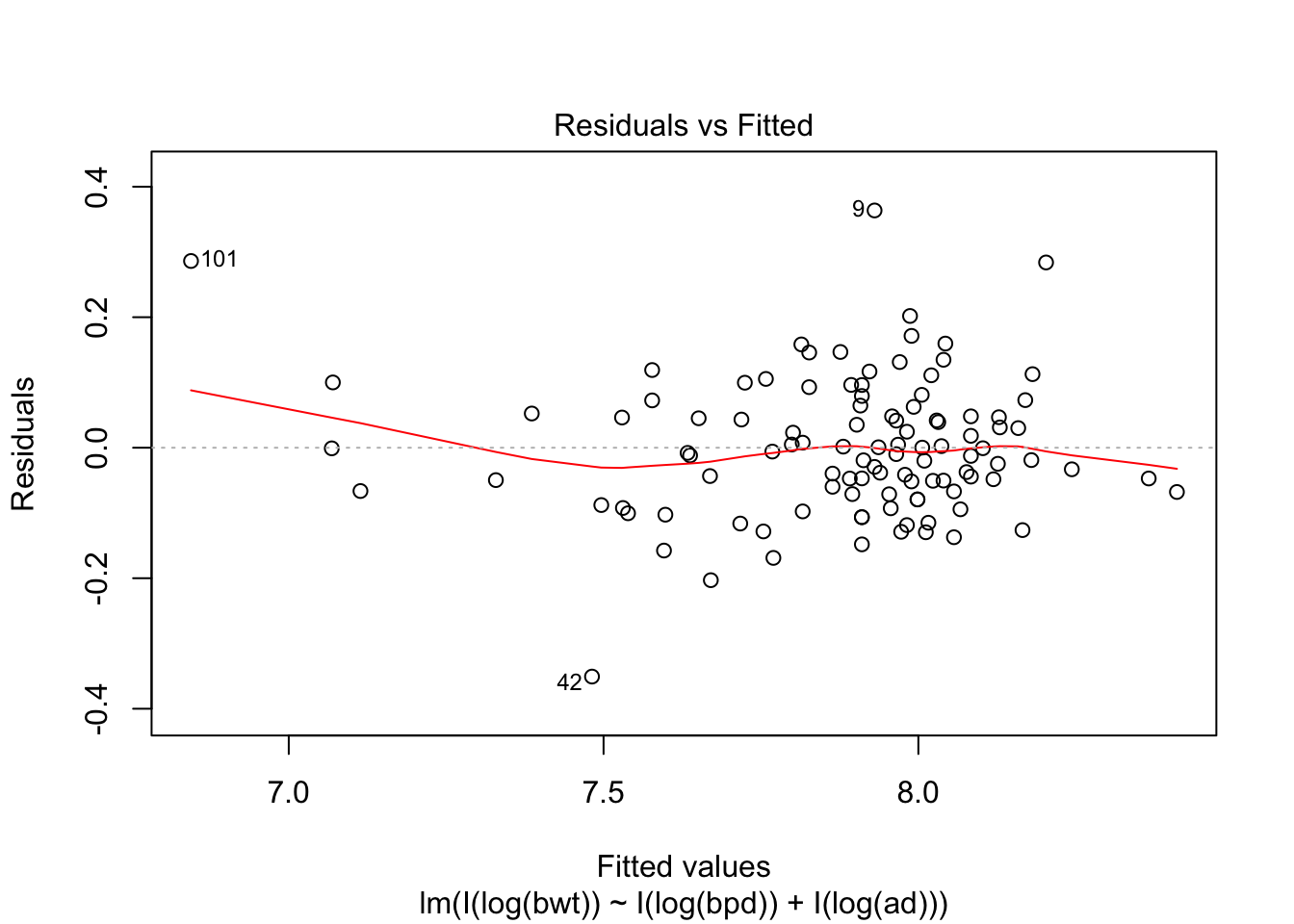
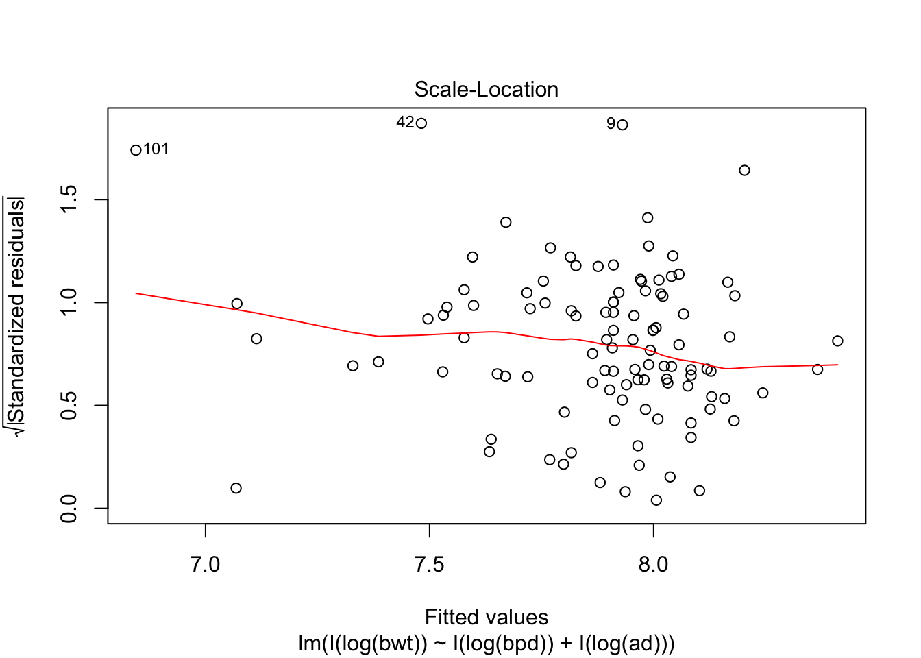
 Looking at the residuals, there seems to be one possible outlier, which is data point 101.
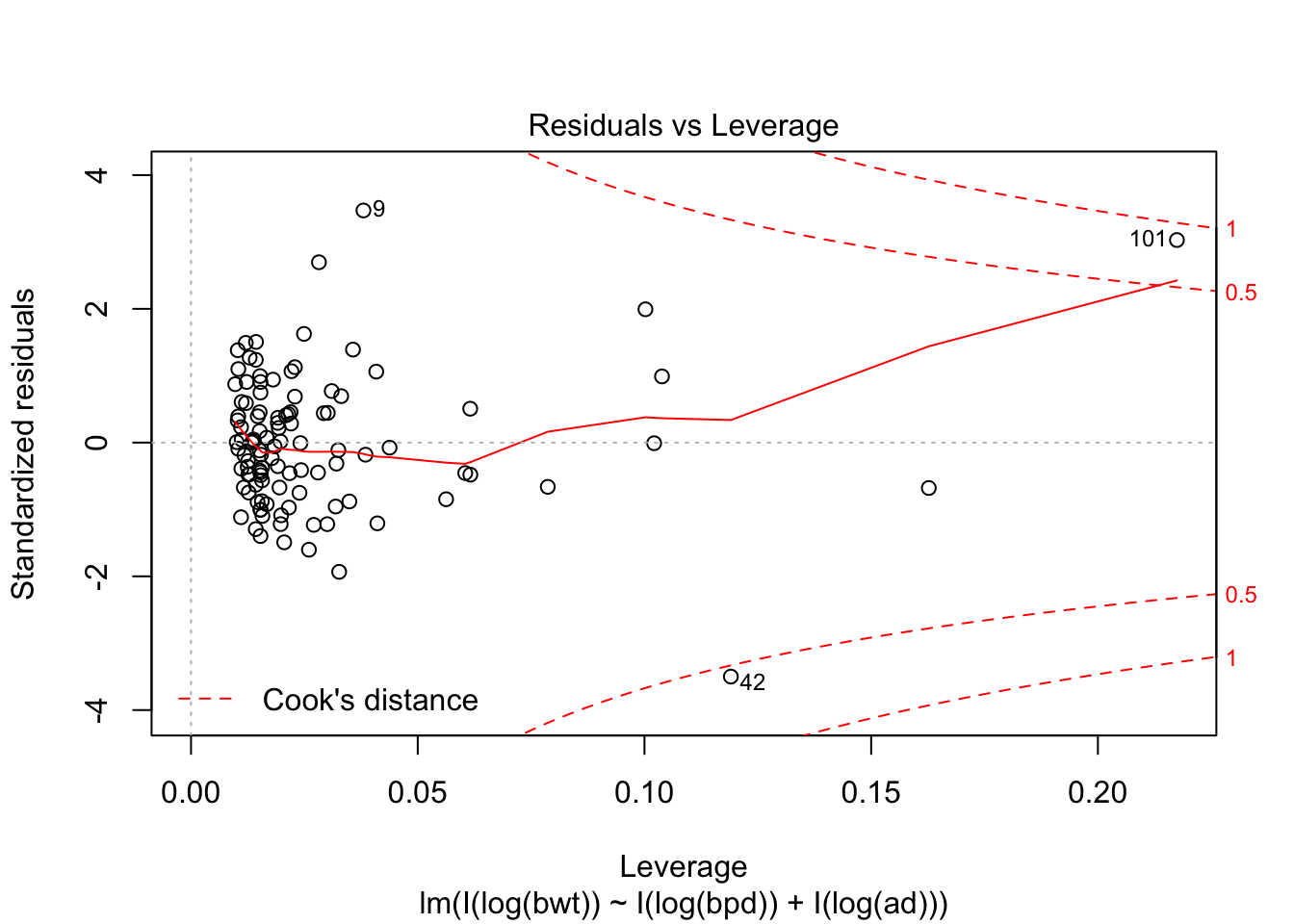
secher[101,]## bwt bpd ad
## 101 1250 64 71summary(secher)## bwt bpd ad
## Min. :1150 Min. : 64.00 Min. : 71.0
## 1st Qu.:2400 1st Qu.: 88.00 1st Qu.: 96.0
## Median :2800 Median : 91.00 Median :103.0
## Mean :2739 Mean : 89.48 Mean :101.7
## 3rd Qu.:3125 3rd Qu.: 93.00 3rd Qu.:108.0
## Max. :4850 Max. :100.00 Max. :133.0We see that the high leverage point is the minimum for both perimeters, and almost the minimum for birthweight. This could be an indication that our model doesn’t hold well for babies whose mothers have small perimeters. Referring back to our original plots of the log transformed data, it is definitely plausible that the model might break down near log(bpd) = 4.3. We certainly have very little data in that range, so our model would be somewhat suspect in that range even if the fit were a little bit better. As it is, I would be hesitant to apply the model to predict infant birth weight for mothers whose log(bpd) is less than 4.3, pending further verification.
For comparison’s sake, let’s see what happens if we only use ad or bpd.
my.mod2 <- lm(I(log(bwt))~I(log(ad)), data = secher)
summary(my.mod2)
##
## Call:
## lm(formula = I(log(bwt)) ~ I(log(ad)), data = secher)
##
## Residuals:
## Min 1Q Median 3Q Max
## -0.58560 -0.06609 0.00184 0.07479 0.48435
##
## Coefficients:
## Estimate Std. Error t value Pr(>|t|)
## (Intercept) -2.4446 0.5103 -4.791 5.49e-06 ***
## I(log(ad)) 2.2365 0.1105 20.238 < 2e-16 ***
## ---
## Signif. codes: 0 '***' 0.001 '**' 0.01 '*' 0.05 '.' 0.1 ' ' 1
##
## Residual standard error: 0.1275 on 105 degrees of freedom
## Multiple R-squared: 0.7959, Adjusted R-squared: 0.794
## F-statistic: 409.6 on 1 and 105 DF, p-value: < 2.2e-16plot(my.mod2, which = c(1,3,5))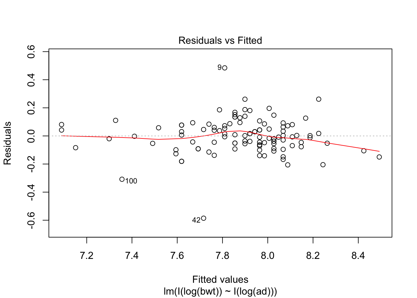
predict(my.mod, newdata = data.frame(bpd = 64, ad = 71))## 1
## 6.84476exp(6.84476)## [1] 938.9479predict(my.mod2, newdata = data.frame(ad = 71))## 1
## 7.0889exp(7.0899)## [1] 1199.788Note that abdominal diameter remains a good predictor for birth weight even in the extreme cases, while biparietal diameter is very far off. Again, we have very little data in this range, so this is all highly speculative.
12.1 Exercises
Consider the data set
tlcin theISwRlibrary. Model the variabletlcinside the data settlcon the other variables. Include plots and examine the residuals.- Load the data set
MRex2.csvfrom http://stat.slu.edu/~speegle/_book_data/MRex2.csv. This data set contains the following variables:- G = The total number of games played in the AL or NL each year.
- HR = The number of home runs hit per game.
- R = The number of runs scored per game.
- SB = The number of stolen bases per game.
- CS = The number of times caught stealing per game.
- IBB = The number of intentional bases on balls per game.
- X2B = The number of doubles hit per game.
- AB = The number of at bats per game.
- PSB = The percentage of time a base stealer was successful.
- yearID = the year in question.
Load the data frame and complete the following tasks:
- Compute the correlation coefficient for each pair of variables. Comment on pairs that are highly correlated.
- Create a scatterplot of Runs scored per game versus each of the other 8 variables.
- Create a linear model of the number of runs scored per game on all of the other variables except
yearID. - CS is considered a bad thing to happen, and leads to fewer runs being scored. Why is the coefficient associated with CS positive?
- Are SB, CS and PSB individually significant?
- Are SB, CS and PSB jointly significant?
- Intelligently remove variables and create a model that describes the response.
- Examine the residuals, and evaluate your model.