7 Hypothesis Testing and Confidence Intervals for the mean

If $X_1,\ldots,X_n$ are iid normal rv’s with mean $\mu$ and standard deviation $\sigma$, then $\overline{X}$ is normal with mean $\mu$ and standard deviation $\sigma/\sqrt{n}$. Then \[ \frac{\overline{X} - \mu}{\sigma/\sqrt{n}} \sim Z \] where $Z$ is standard normal. One can use this information to do computations about probabilities of $\overline{X}$ in the case when $\sigma$ is known. However, many times, $\sigma$ is not known. In that case, we replace $\sigma$ by its estimate based on the data, $S$. The value $S/\sqrt{n}$ is called the standard error of $\overline{X}$. The standard error is no longer the standard deviation of $\overline{X}$, but an approximation that is also a random variable.

The question then becomes: what kind of distribution is \[ \frac{\overline{X} - \mu}{S/\sqrt{n}}? \]

Theorem 7.1 If $X_1,\ldots,X_n$ are iid normal rvs with mean $\mu$ and sd $\sigma$, then \[ \frac{\overline{X} - \mu}{S/\sqrt{n}} \] is $t$ with $n-1$ degrees of freedom.

We will not prove this theorem, but let’s verify through simulation that the pdf’s look similar in some special cases.

Example We simulate the pdf of $\frac{\overline{X} - \mu}{S/\sqrt{n}}$ when $n = 6$, $\mu = 3$ and $\sigma = 4$, and compare to the pdf of a $t$ rv with 3 degrees of freedom.

n <- 6
mu <- 3
sigma <- 4
tData <- replicate(10000, {
  normData <- rnorm(n,mu,sigma);
  (mean(normData) - mu)/(sd(normData)/sqrt(n))
  })
f <- function(x) dt(x,3)
ggplot(data.frame(tData), aes(x = tData)) + 
  geom_density() + 
  stat_function(fun = f, color = "red")

While certainly not a proof, the close match between the simulated values and the $t$-distribution is pretty convincing.

Exercise Simulate the pdf of $\frac{\overline{X} - \mu}{S/\sqrt{n}}$ when $n = 3$, $\mu = 5$ and $\sigma = 1$, and compare to the pdf of a $t$ random variable with 2 degrees of freedom.

Now, suppose that we don’t know either $\mu$ or $\sigma$, but we do know that our data is randomly sampled from a normal distribution. Let $t_{\alpha}$ be the unique real number such that $P(t > t_{\alpha}) = \alpha$, where $t$ has $n-1$ degrees of freedom. Note that $t_{\alpha}$ depends on $n$, because the $t$ distribution has more area in its tails when $n$ is small.

Then, we know that \[ P\left( t_{1 - \alpha/2} < \frac{\overline{X} - \mu}{S/\sqrt{n}} < t_{\alpha/2}\right) = \alpha. \]

By rearranging, we get

\[ P\left(\overline{X} + t_{1 - \alpha/2} S/\sqrt{n} < \mu < \overline{X} + t_{\alpha/2} S/\sqrt{n}\right) = 1 - \alpha. \]

Because the $t$ distribution is symmetric, $t_{1-\alpha/2} = -t_{\alpha/2}$, so we can rewrite the equation symmetrically as:

\[ P\left(\overline{X} - t_{\alpha/2} S/\sqrt{n} < \mu < \overline{X} + t_{\alpha/2} S/\sqrt{n}\right) = 1 - \alpha. \]

Let’s think about what this means. Take $n = 10$ and $\alpha = 0.10$ just to be specific. This means that if I were to repeatedly take 10 samples from a normal distribution with mean $\mu$ and any $\sigma$, then 90% of the time, $\mu$ would lie between $\overline{X} + t_{\alpha/2} S/\sqrt{n}$ and $\overline{X} - t_{\alpha/2} S/\sqrt{n}$. That sounds like something that we need to double check using a simulation!

t05 <- qt(.05, 9, lower.tail = FALSE)
mean(replicate(10000, {
  dat <- rnorm(10,5,8);
  xbar <- mean(dat);
  SE <- sd(dat)/sqrt(10);
  ( xbar - t05 * SE < 5 ) & ( xbar + t05 * SE > 5 )
}))

The first line computes $t_{\alpha/2}$ using qt, the quantile function for the $t$ distribution, here with 9 DF. Then we check the inequality given above.

Think carefully about what value you expect to get here, then copy this code into R and run it. Were you right?

Exercise Repeat the above simulation with $n = 20$, $\mu = 7$ and $\alpha = .05$.

7.1 Confidence intervals for the mean

If we take a sample of size $n$ from iid normal random variables, then we call the interval

\[ \left[ \overline{X} - t_{\alpha/2} S/\sqrt{n},\ \ \overline{X} + t_{\alpha/2} S/\sqrt{n} \right] \] a 100(1 - $\alpha$)% confidence interval for $\mu$. As we saw in the simulation above, what this means is that if we repeat this experiment many times, then in the limit 100(1 - $\alpha$)% of the time, the mean $\mu$ will lie in the confidence interval. Of course, once we have done the experiment and we have an interval, it doesn’t make sense to talk about the probability that $\mu$ (a constant) is in the (constant) interval. There is nothing random there. However, we can say that we are 100(1 - $\alpha$)% confident that the mean is in the interval.

As you might imagine, R has a built in command that does all of this for us. Consider the heart rate and body temperature data normtemp.⁵

You can read normtemp from a file as follows, assuming the file is stored in the same directory as is returned when you type getwd(), or get it from the UsingR package.

normtemp <- read.csv("normtemp.csv")

What kind of data is this?

str(normtemp)

## 'data.frame':    130 obs. of  3 variables:
##  $ Gender    : Factor w/ 2 levels "Female","Male": 2 2 2 2 2 2 2 2 2 2 ...
##  $ Body.Temp : num  96.3 96.7 96.9 97 97.1 97.1 97.1 97.2 97.3 97.4 ...
##  $ Heart.Rate: int  70 71 74 80 73 75 82 64 69 70 ...

head(normtemp)

##   Gender Body.Temp Heart.Rate
## 1   Male      96.3         70
## 2   Male      96.7         71
## 3   Male      96.9         74
## 4   Male      97.0         80
## 5   Male      97.1         73
## 6   Male      97.1         75

We see that the data set is 130 observations of body temperature and heart rate. There is also gender information attached, that we will ignore for the purposes of this example.

Let’s find a 98 confidence interval for the mean heart rate of healthy adults. In order for this to be valid, we are assuming that we have a random sample from all healthy adults (highly unlikely to be formally true), and that the heart rate of healthy adults is normally distributed (also unlikely to be formally true). Later, we will discuss deviations from our assumptions and when we should be concerned.

The R command that finds a confidence interval for the mean in this way is

t.test(normtemp$Heart.Rate, conf.level = .98)

## 
##  One Sample t-test
## 
## data:  normtemp$Heart.Rate
## t = 119.09, df = 129, p-value < 2.2e-16
## alternative hypothesis: true mean is not equal to 0
## 98 percent confidence interval:
##  72.30251 75.22056
## sample estimates:
## mean of x 
##  73.76154

We get a lot of information, but we can pull out what we are looking for as the confidence interval [72.3, 75.2]. So, we are 98 confident that the mean heart rate of healthy adults is greater than 72.3 and less than 75.2. NOTE We are not saying anything about the mean heart rate of the people in the study. That is exactly 73.76154, and we don’t need to do anything fancy. We are making an inference about the mean heart rate of all healthy adults. Note that to be more precise, we might want to say it is the mean heart rate of all healthy adults as would be measured by this experimenter. Other experimenters could have a different technique for measuring hear rates which would lead to a different answer. It is traditional to omit that statement from conclusions, though you might consider its implications in the following exercise.

Exercise Find a 99 confidence interval for the mean body temperature of healthy adults. Before you start, do you expect the interval to contain the value 98.6? (That is the accepted normal body temperature of adults in Fahrenheit, which could be useful information to you if you are ever traveling in the US!)

7.2 Hypothesis Tests of the Mean

In hypothesis testing, there is a null hypothesis and an alternative hypothesis. The null hypothesis can take on several forms: that a population is a specified value, that two population parameters are equal, that two population distributions are equal, and many others. The common thread being that it is a statement about the population distribution. Typically, the null hypothesis is the default assumption, or the conventional wisdom about a population. Often it is exactly the thing that a researcher is trying to show is false. The alternative hypothesis states that the null hypothesis is false, sometimes in a particular way.

Consider as an example, the body temperature of healthy adults, as in the previous subsection. The natural choice for the null and alternative hypothesis is

$H_0: \, \mu = 98.6$ versus

$H_a: \, \mu \not= 98.6$.

We will either reject $H_0$ in favor of $H_a$, or we will not reject $H_0$ in favor of $H_a$. (Note that this is different than accepting $H_0$.) There are two types of errors that can be made: Type I is when you reject $H_0$ when $H_0$ is actually true, and Type II is when you fail to reject $H_0$ when $H_a$ is actually true. For now, we will worry about controlling the probability of a Type I error.

In order to compute the probability of a type I error, we imagine that we collect the same type of data many times, when $H_0$ is actually true. If we decide on rejecting $H_0$ whenever it falls in a certain rejection region (RR), then the probability of a type I error would be the probability that the data falls in the rejection region given that $H_0$ is true.

Returning to the specifics of $H_0: \mu = \mu_0$ versus $H_a: \mu \not= \mu_0$, we compute the test statistic \[ T = \frac{\overline{X} - \mu}{S/\sqrt{n}} \] And we ask: if I decide to reject $H_0$ based on this test statistic, what percentage of the time would I get data at least that much against $H_0$ even though $H_0$ is true? In other words, if I decide to reject $H_0$ based on $T$, I would have to reject $H_0$ for any data that is even more compelling against $H_0$. Howe often would that happen under $H_0$? Well, that is what the $p$-value is. In this case, it is

t.test(normtemp$Body.Temp, mu = 98.6)

## 
##  One Sample t-test
## 
## data:  normtemp$Body.Temp
## t = -5.4548, df = 129, p-value = 2.411e-07
## alternative hypothesis: true mean is not equal to 98.6
## 95 percent confidence interval:
##  98.12200 98.37646
## sample estimates:
## mean of x 
##  98.24923

I get a $p$-value of about 0.000002, which is the probability that I would get data at least this compelling against $H_0$ even though $H_0$ is true. In other words, it is very unlikely that this data would be collected if the true mean temp of healthy adults is 98.6. (Again, we are assuming a random sample of healthy adults and normal distribution of temperatures of healthy adults.)

Let’s look at another example. Altman (1991) measured the daily energy (KJ) intake of 11 women. Let’s store it in

library(ISwR)
daily.intake <- intake$pre

It is recommended that women consume 7725 KJ per day. Is there evidence to suggest that women do not consume the recommended amount? Find a 99% confidence interval for the daily energy intake of women.

We need to assume that this is a random sample of 11 women from some population. We are making statements about the group of women that these 11 were sampled from. If they were 11 randomly selected patients of Dr.~Altman, then we are making statements about patients of Dr.~Altman. We also need to assume that energy intake is normally distributed, which seems a reasonable enough assumption. Then, we compute

t.test(daily.intake, mu = 7725, conf.level = .99)

## 
##  One Sample t-test
## 
## data:  daily.intake
## t = -2.8208, df = 10, p-value = 0.01814
## alternative hypothesis: true mean is not equal to 7725
## 99 percent confidence interval:
##  5662.256 7845.017
## sample estimates:
## mean of x 
##  6753.636

We see that the 99% confidence interval is $(5662,7845)$, and the $p$-value is .01814. So, there is about a 1.8% chance of getting data that is this compelling or more against $H_0$ even if $H_0$ is true.

We would reject $H_0$ at the $\alpha = .05$ level, but fail to reject at the $\alpha = .01$ level. For the purposes of this book, the $\alpha$ level will usually be specified in a problem, but if it isn’t, then you are free to choose a reasonable level based on the type of problem that we are talking about. Common choices are $\alpha = .01$ and $\alpha = .05$.

7.3 One-sided Confidence Intervals and Hypothesis Tests

Consider the data set anorexia, in the MASS library. Since we do not need the entire MASS package and MASS has a function select that interferes with the dplyr function that we use a lot, let’s just load the data from MASS into a variable called anorexia without loading the entire MASS package.

anorexia <- MASS::anorexia

This data set consists of pre- and post- treatment measurements for anorexia patients. There are three different treatments of patients, which we ignore in this example (we will come back to that later in the class). In this case, we have reason to believe that the medical treatment that the patients are undergoing will result in an increased weight. So, we are not as much interested in detecting a change in weight, but an increase in weight. This changes our analysis.

We will construct a 98% confidence interval for the variable weightdifference of the form $(L, \infty)$. We will say that we are 98% confident that the treatment results in a mean change of weight of at least $L$ pounds. As before, this interval will be constructed so that 98% of the time that we perform the experiment, the true mean will fall in the interval (and 2% of the time, it will not). As before, we are assuming normality of the underlying population. We will also perform the following hypothesis test:

$H_0: \mu \le 0$ vs

$H_a: \mu > 0$

There is no practical difference between $H_0: \mu \le 0$ and $H_0: \mu = 0$ in this case, but knowing the alternative is $\mu > 0$ makes a difference. Now, the evidence that is most in favor of $H_a$ is all of the form $\overline{x} > L$. So, the percent of time we would make a type I error under $H_0$ is \[ P(\frac{\overline{X} - \mu_0}{S/\sqrt{n}} > L) \] where $\mu_0 = 0$ in this case. After collecting data, if we reject $H_0$, we would also have rejected $H_0$ if we got more compelling evidence against $H_0$, so we would compute \[ P(t_{n-1} > \frac{\overline{x} - \mu_0}{S/\sqrt{n}}) \] where $\frac{\overline{x} - \mu_0}{S/\sqrt{n}}$ is the value computed from the data. R does all of this for us:

weightdifference <- anorexia$Postwt - anorexia$Prewt
t.test(weightdifference, mu = 0, alternative = "greater", conf.level = .98)

## 
##  One Sample t-test
## 
## data:  weightdifference
## t = 2.9376, df = 71, p-value = 0.002229
## alternative hypothesis: true mean is greater than 0
## 98 percent confidence interval:
##  0.7954181       Inf
## sample estimates:
## mean of x 
##  2.763889

There is pretty strong evidence that there is a positive mean difference in weight of patients.

7.4 Simulations

In the chapter up to this point, we have assumed that the underlying data is a random sample from a normal distribution. Let’s look at how various types of departures from that assumption affect the validity of our statistical procedures. For the purposes of this discussion, we will restrict to hypothesis testing at a specified $\alpha$ level, but our results will hold for confidence intervals and reporting $p$-values just as well.

Our point of view is that if we design our hypothesis test at the $\alpha = .1$ level, say, then we want to incorrectly reject the null hypothesis 10% of the time. That is how our test is designed. If our assumptions of normality are violated, then we want to measure the new effective type I error rate and compare it to 10%. If the new error rate is far from 10%, then the test is not performing as designed. We will note whether the test makes too many type I errors or too few, but the main objective is to see whether the test is performing as designed.

Our first observation is that when the sample size is large, then the central limit theorem tells us that $\overline{X}$ is approximately normal. Since $t_n$ is also approximately normal when $n$ is large, this gives us some measure of protection against departures from normality in the underlying population. It will be very useful to pull out the $p$-value of the t.test. Let’s see how we can do that. We begin by doing a t.test on “garbage data” just to see what t.test returns.

str(t.test(c(1,2,3)))

## List of 9
##  $ statistic  : Named num 3.46
##   ..- attr(*, "names")= chr "t"
##  $ parameter  : Named num 2
##   ..- attr(*, "names")= chr "df"
##  $ p.value    : num 0.0742
##  $ conf.int   : atomic [1:2] -0.484 4.484
##   ..- attr(*, "conf.level")= num 0.95
##  $ estimate   : Named num 2
##   ..- attr(*, "names")= chr "mean of x"
##  $ null.value : Named num 0
##   ..- attr(*, "names")= chr "mean"
##  $ alternative: chr "two.sided"
##  $ method     : chr "One Sample t-test"
##  $ data.name  : chr "c(1, 2, 3)"
##  - attr(*, "class")= chr "htest"

It’s a list of 9 things, and we can pull out the $p$-value by using t.test(c(1,2,3))$p.value.

7.4.1 Symmetric, light tailed

Example Estimate the effective type I error rate in a t-test of $H_0: \mu = 0$ versus $H_a: \mu\not = 0$ at the $\alpha = 0.1$ level when the underlying population is uniform on the interval $(-1,1)$ when we take a sample size of $n = 10$.

Note that $H_0$ is definitely true in this case. So, we are going to estimate the probability of rejecting $H_0$ under the scenario above, and compare it to 10%, which is what the test is designed to give. Let’s build up our replicate function step by step.

set.seed(1)
runif(10,-1,1) #Sample of size 10 from uniform rv

##  [1] -0.4689827 -0.2557522  0.1457067  0.8164156 -0.5966361  0.7967794
##  [7]  0.8893505  0.3215956  0.2582281 -0.8764275

t.test(runif(10,-1,1))$p.value #p-value of test

## [1] 0.5089686

t.test(runif(10,-1,1))$p.value < .1 #true if we reject

## [1] FALSE

mean(replicate(10000, t.test(runif(10,-1,1))$p.value < .1))

## [1] 0.1007

Our result is 10.07%. That is really close to the designed value of 10%.

Exercise Repeat the above example for various values of $\alpha$ and $n$. How big does $n$ need to be for the t.test to give results close to how it was designed? (Note: there is no one right answer to this ill-posed question! There are, however, wrong answers. The important part is the process you use to investigate.)

7.4.2 Skew

Example Estimate the effective type I error rate in a t-test of $H_0: \mu = 1$ versus $H_a: \mu\not = 1$ at the $\alpha = 0.05$ level when the underlying population is exponential with rate 1 when we take a sample of size $n = 20$.

set.seed(2)
mean(replicate(20000, t.test(rexp(20,1), mu = 1)$p.value < .05))

## [1] 0.08305

Note that we have to specify the null hypothesis mu = 1 in the t.test. Here we get an effective type I error rate (rejecting $H_0$ when $H_0$ is true) that is 3.035 percentage points higher than designed. This means our error rate will increase by 61%. Most people would argue that the test is not working as designed.

One issue is the following: how do we know we have run replicate enough times to get a reasonable estimate for the probability of a type I error? Well, we don’t. If we repeat our experiment a couple of times, though, we see that we get consistent results, which for now we will take as sufficient evidence that our estimate is closer to correct.

mean(replicate(20000, t.test(rexp(20,1), mu = 1)$p.value < .05))

## [1] 0.08135

mean(replicate(20000, t.test(rexp(20,1), mu = 1)$p.value < .05))

## [1] 0.0836

Pretty similar each time. That’s reason enough for me to believe the true type I error rate is relatively close to what we computed.

We summarize the simulated effective Type I error rates for $H_0: \mu = 1$ versus $H_a: \mu \not= 1$ at $\alpha = .1, .05, .01$ and $.001$ levels for sample sizes $N = 10, 20, 50, 100$ and 200.

effectiveError <- sapply(c(.1,.05,.01,.001), function (y) sapply(c(10,20,50,100,200), function(x) mean(replicate(20000, t.test(rexp(x,1), mu = 1)$p.value < y))  ))
colnames(effectiveError) <- c(".1", ".05", ".01", ".001")
rownames(effectiveError) <- c("10", "20", "50", "100", "200")
tbl_df(effectiveError)

## # A tibble: 5 x 4
##      `.1`   `.05`   `.01`  `.001`
##     <dbl>   <dbl>   <dbl>   <dbl>
## 1 0.14385 0.09620 0.04700 0.01440
## 2 0.13045 0.08260 0.03270 0.01195
## 3 0.11230 0.06735 0.02160 0.00745
## 4 0.10900 0.05885 0.01795 0.00450
## 5 0.10510 0.05450 0.01395 0.00255

Exercise Repeat the above example for exponential rv’s when you have a sample size of 150 for $\alpha = .1$, $\alpha = .01$ and $\alpha = .001$. I recommend increasing the number of times you are replicating as $\alpha$ gets smaller. Don’t go crazy though, because this can take a while to run.

From the previous exercise, you should be able to see that at $n = 50$, the effective type I error rate gets worse in relative terms as $\alpha$ gets smaller. (For example, my estimate at the $\alpha = .001$ level is an effective error rate more than 6 times what is designed! We would all agree that the test is not performing as designed.) That is unfortunate, because small $\alpha$ are exactly what we are interested in! That’s not to say that t-tests are useless in this context, but $p$-values should be interpreted with some level of caution when there is thought that the underlying population might be exponential. In particular, it would be misleading to report a $p$-value with 7 significant digits in this case, as R does by default, when in fact it is only the order of magnitude that is significant. Of course, if you know your underlying population is exponential before you start, then there are techniques that you can use to get accurate results which are beyond the scope of this textbook.

7.4.3 Heavy tails and outliers

If the results of the preceding section didn’t convince you that you need to understand your underlying population before applying a t-test, then this section will. A typical “heavy tail” distribution is the $t$ random variable. Indeed, the $t$ rv with 1 or 2 degrees of freedom doesn’t even have a finite standard deviation!

Example Estimate the effective type I error rate in a t-test of $H_0: \mu = 0$ versus $H_a: \mu\not = 0$ at the $\alpha = 0.1$ level when the underlying population is $t$ with 3 degrees of freedom when we take a sample of size $n = 30$.

mean(replicate(20000, t.test(rt(30,3), mu = 0)$p.value < .1))

## [1] 0.09735

Not too bad. It seems that the t-test has an effective error rate less than how the test was designed.

Example Estimate the effective type I error rate in a t-test of $H_0: \mu = 3$ versus $H_a: \mu\not = 3$ at the $\alpha = 0.1$ level when the underlying population is normal with mean 3 and standard deviation 1 with sample size $n = 100$. Assume however, that there is an error in measurement, and one of the values is multiplied by 100 due to a missing decimal point.

mean(replicate(20000, t.test(c(rnorm(99, 3, 1),100*rnorm(1, 3, 1)), mu = 3)$p.value < .1))

## [1] 1e-04

These numbers are so small, it makes more sense to sum them:

sum(replicate(20000, t.test(c(rnorm(99, 3, 1),100*rnorm(1, 3, 1)), mu = 3)$p.value < .1))

## [1] 3

So, in this example, you see that we would reject $H_0$ 3 out of 20,000 times, when the test is designed to reject it 2,000 times out of 20,000! You might as well not even bother running this test, as you are rarely, if ever, going to reject $H_0$ even when it is false.

Example Estimate the percentage of time you would correctly reject $H_0: \mu = 7$ versus $H_a: \mu\not = 7$ at the $\alpha = 0.1$ level when the underlying population is normal with mean 3 and standard deviation 1 with sample size $n = 100$. Assume however, that there is an error in measurement, and one of the values is multiplied by 100 due to a missing decimal point.

Note that here, we have a null hypothesis that is 4 standard deviations away from the true null hypothesis. That should be easy to spot. Let’s see.

mean(replicate(20000, t.test(c(rnorm(99, 3, 1),100*rnorm(1, 3, 1)), mu = 7)$p.value < .1))

## [1] 0.0711

There is no “right” value to compare this number to. We have estimated the probability of correctly rejecting a null hypothesis that is 4 standard deviations away from the true value (which is huge!!) as 0.0722. So, we would only detect a difference that large about 7% of the time that we run the test. That’s hardly worth doing.

7.4.4 Summary

When doing t-tests on populations that are not normal, the following types of departures from design were noted.

When the underlying distribution is skew, the exact $p$-values should not be reported to many significant digits (especially the smaller they get). If a $p$-value close to the $\alpha$ level of a test is obtained, then we would want to note the fact that we are unsure of our $p$-values due to skewness, and fail to reject.
When the underlying distribution has outliers, the power of the test is severely compromised. A single outlier of sufficient magnitude will force a t-test to never reject the null hypothesis. If your population has outliers, you do not want to use a t-test.

7.5 Two sample hypothesis tests of $\mu_1 = \mu_2$

Here, we present a couple of examples of two sample t tests. In this situation, we have two populations that we are sampling from, and we are wondering whether the mean of population one differs from the mean of population two. At least, that is the problem we are typically working on!

The assumptions for t tests remain the same. We are assuming that the underlying populations are normal, or that we have enough samples so that the central limit theorem takes hold. We are also AS ALWAYS assuming that there are no outliers. Remember: outliers can kill t tests. Both the one-sample and the two-sample variety.

We also have two other choices.

We can assume that the variances of the two populations are equal. If the variances of the two populations really are equal, then this is the correct thing to do. In general, it is a more conservative approach not to assume the variances of the two populations are equal, and I generally recommend not to assume equal variance unless you have a good reason for doing so.
Whether the data is paired or unpaired. Paired data results from multiple measurements of the same individual at different times, while unpaired data results from measurements of different individuals. Say, for example, you wish to determine whether a new fertilizer increases the mean number of apples that apple trees produce. If you count the number of apples one season, and then the next season apply the fertilizer and count the number of apples again, then you would expect there to be some relationship between the number of apples you count in each season (big trees would have more apples each season than small trees, for example). If you randomly selected half of the trees to apply fertilizer to in one growing season, then there would not be any dependencies in the data.In general, it is a hard problem to deal with dependent data, but paired data is one type of data that we can deal with.

Example (This example requires the ISwR library.) Consider the igf1 levels of girls in tanner puberty levels I and V. Test whether the mean igf1 level is the same in both populations.

Let $\mu_1$ be the mean igf1 level of all girls in tanner puberty level I, and let $\mu_2$ be the mean igf1 level of all girls in tanner puberty level V. We wish to test

\[ H_0: \mu_1 = \mu_2 \] versus \[ H_a: \mu_1\not= \mu_2 \]

Let’s think about the data that we have for a minute. Do we expect the igf1 level of girls in the two puberty levels to be approximately normal? Do we expect symmetry? How many samples do we have?

juul <- ISwR::juul

We need to clean up the juul data:

juul$sex <- factor(juul$sex, levels = c(1,2), labels = c("Boy", "Girl"))
juul$menarche <- factor(juul$menarche, levels = c(1,2), labels = c("No", "Yes"))
juul$tanner <- factor(juul$tanner, levels = c(1,2,3,4,5), labels = c("I", "II", "III", "IV", "V"))

Now let’s see what our sample sizes are:

table(juul$sex, juul$tanner)

##       
##          I  II III  IV   V
##   Boy  291  55  34  41 124
##   Girl 224  48  38  40 204

And we can see that we have 224 girls in tanner I and 204 in tanner V. I doubt that the data would be so skewed that we would need to worry about using t test in this case. I also don’t think there will be outliers.

We can get a boxplot of all of the girls in tanner 1 or 5’s igf1 levels. Let’s create a data frame that consists only of those observations that are girls in tanner 1 or tanner 5.

smallJuul <- dplyr::filter(juul, tanner %in% c("I","V"), sex == "Girl")

ggplot(smallJuul, aes(x = tanner, y = igf1)) + geom_boxplot()

## Warning: Removed 119 rows containing non-finite values (stat_boxplot).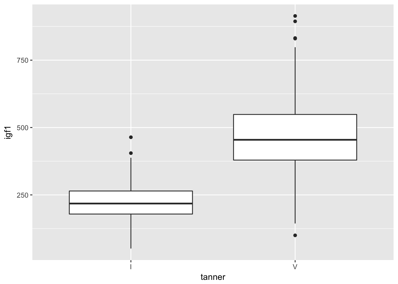

Looks pretty symmetric, and the outliers aren’t too far away from the whiskers. It looks like we were correct to assume that t test will be applicable to this data. Moreover, we had no reason before collecting the data to think that the variances were equal, so we will not make that assumption in t.test. Finally, before collecting the data, we had no reason to believe that the igf1 levels of the two populations would differ in a particular way, so we do a 2-sided test.

Now, we run a t-test:

t.test(igf1~tanner, data = smallJuul, var.equal = FALSE)

## 
##  Welch Two Sample t-test
## 
## data:  igf1 by tanner
## t = -19.371, df = 290.68, p-value < 2.2e-16
## alternative hypothesis: true difference in means is not equal to 0
## 95 percent confidence interval:
##  -266.5602 -217.3884
## sample estimates:
## mean in group I mean in group V 
##        225.2941        467.2684

OK, that’s crazy. We definitely reject $H_0$. Looking back at the boxplots, notice that the 25th percentile of the tanner 5 girls is almost above the whisker of the tanner 1 girls. That’s a pretty huge difference, and we almost didn’t even need to run a t test.

7.5.1 Example Two

Consider the data in anorexia in the MASS library. Is there sufficient evidence to conclude that there is a difference in the pre- and post- treatment weights of girls receiving the CBT treatment?

Formally, we let $\mu_1$ denote the mean pre-treatment weight of girls with anorexia, and we let $\mu_2$ denote the mean post-CBT treatment weight of girls with anorexia. We test \[ H_0: \mu_1 = \mu_2 \] versus \[ H_a: \mu_1 < \mu_2 \] We choose a one-sided test because we have reason to believe that the CBT treatment will help the girls gain weight, and I am doing so before looking at the data. I will not reject the null hypothesis if it turns out that the post treatment weight is less than the pre treatment weight.

Additionally, since we are doing repeated measurements on the same individuals, this data is paired and dependent. We will need to include paired = TRUE when we call t.test.

The assumptions of t tests are: the pre and post treatment weights are normally distributed (we can do less than that in this case, since we have paired data, but…), or that the population is close enough to normal for the sample size that we have, and that the weights are independent (except for being paired). I am willing to make those assumptions for this experiment. The data is plotted below; please take a look at the plots.

anorexia <- MASS::anorexia
anorexia <- filter(anorexia, Treat == "CBT")
str(anorexia)

## 'data.frame':    29 obs. of  3 variables:
##  $ Treat : Factor w/ 3 levels "CBT","Cont","FT": 1 1 1 1 1 1 1 1 1 1 ...
##  $ Prewt : num  80.5 84.9 81.5 82.6 79.9 88.7 94.9 76.3 81 80.5 ...
##  $ Postwt: num  82.2 85.6 81.4 81.9 76.4 ...

Looks good. Let’s run the test.

t.test(anorexia$Prewt,anorexia$Postwt, paired = TRUE, alternative = "less")

## 
##  Paired t-test
## 
## data:  anorexia$Prewt and anorexia$Postwt
## t = -2.2156, df = 28, p-value = 0.01751
## alternative hypothesis: true difference in means is less than 0
## 95 percent confidence interval:
##        -Inf -0.6981979
## sample estimates:
## mean of the differences 
##               -3.006897

We see that we get a p-value of 0.01751. That is evidence that the treatment has been effective. Note that if we didn’t pair the data, we would get

t.test(anorexia$Prewt,anorexia$Postwt,alternative = "less")

## 
##  Welch Two Sample t-test
## 
## data:  anorexia$Prewt and anorexia$Postwt
## t = -1.677, df = 44.931, p-value = 0.05024
## alternative hypothesis: true difference in means is less than 0
## 95 percent confidence interval:
##         -Inf 0.004459683
## sample estimates:
## mean of x mean of y 
##  82.68966  85.69655

which has a p-value of .05024. That is, the p-value would be three times as large.

Finally, let’s look at the data to make sure no outliers snuck in.

ggplot(anorexia, aes(x = "", y = Prewt)) + geom_boxplot()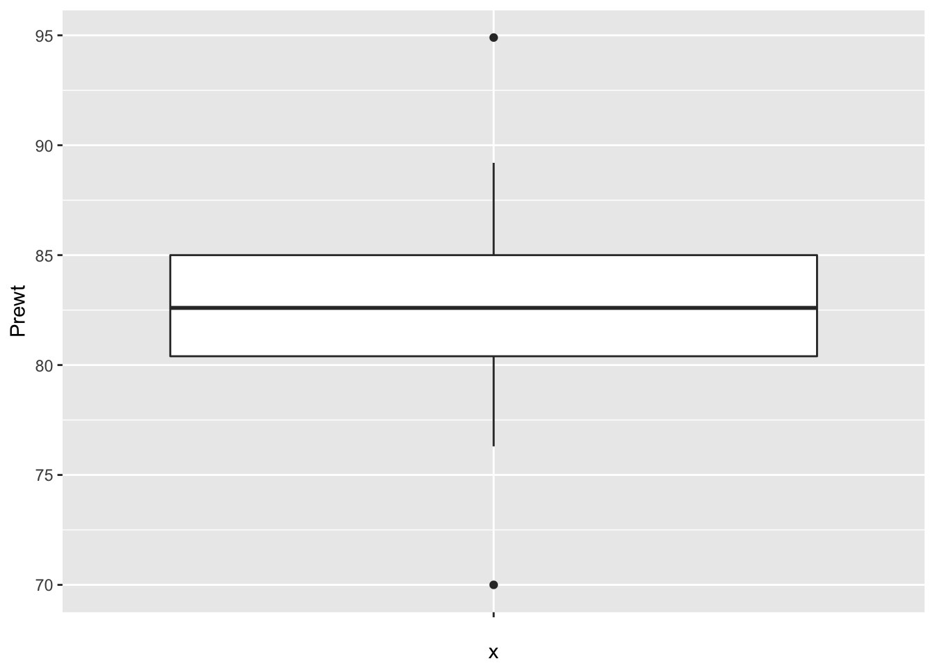

ggplot(anorexia, aes(x = "", y = Postwt)) + geom_boxplot()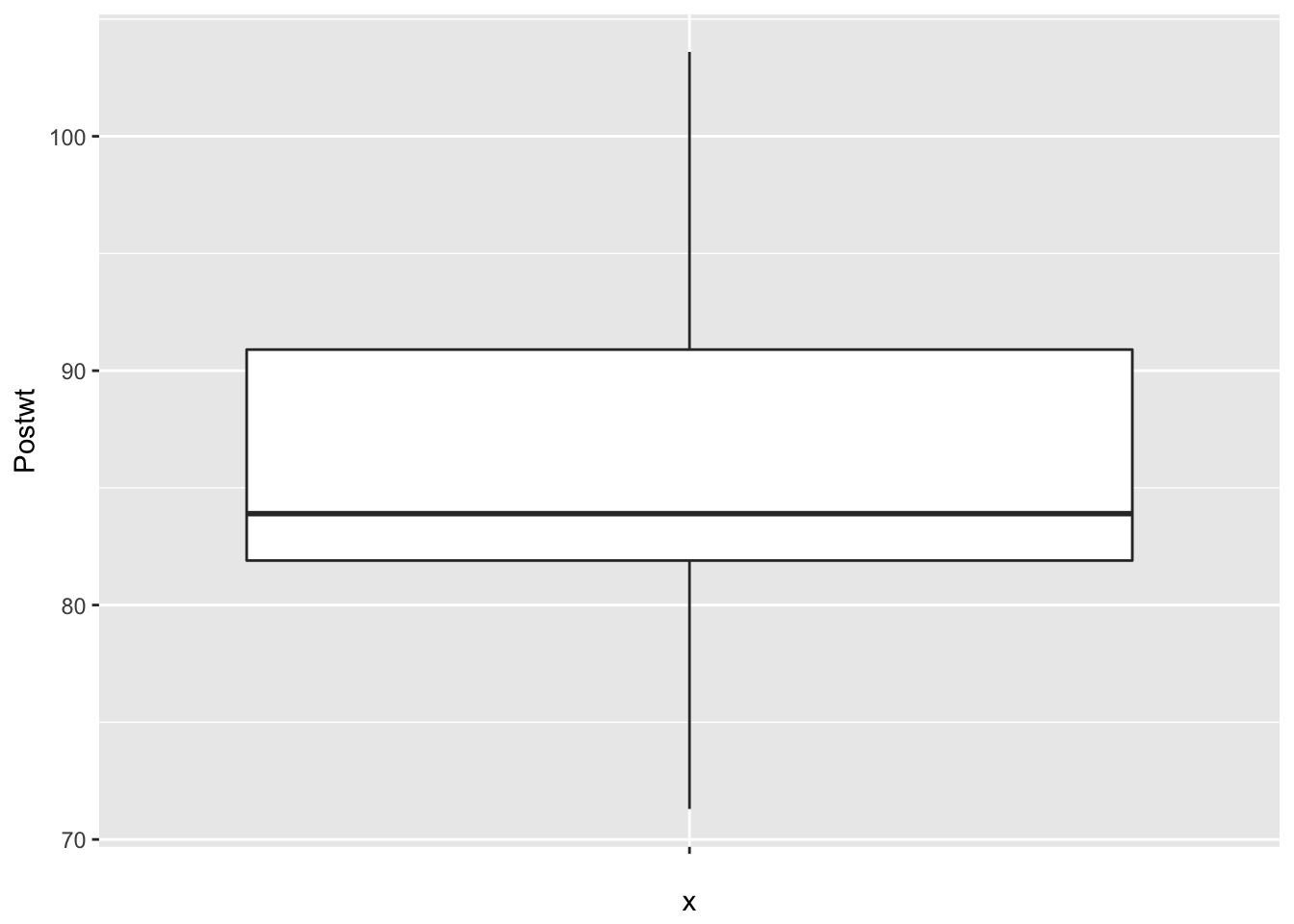

It is interesting that the pre-treatment weights are nice and symmetric, while the post-treatment weights are skew. This leads me to wonder whether the treatment wasn’t effective for all of the patients, and maybe there is some subset of patients for which this treatment tends to work. Without further information, we won’t be able to tell.

ggplot(anorexia, aes(x = Postwt - Prewt)) + geom_histogram(binwidth = 5)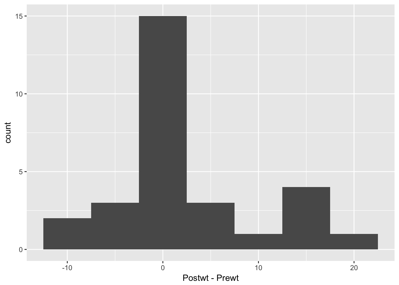

Looking at this, it seems that the treatment was totally ineffective for some girls, but almost unrealistically effective for some others. I would really like to understand which patients are more likely to be helped by this treatment. But, we don’t have any data that would help us to understand it. Perhaps we should submit a grant proposal…

7.6 Exercises

Use the built in R dataset precip to compute a 99% confidence interval for the mean rainfall in US cities.
Michelson’s measurements of the speed of light. Get the file data/michelson_light_speed.csv. This file contains two series of measurements of the speed of light made by Albert Michelson in 1879 and 1882. The measurements are given in amounts over 299000 km/s.
1. Find a 95% confidence interval for the speed of light using the 1879 data.
2. Find a 95% confidence interval for the speed of light using the 1882 data.
3. Which set of data has a higher SD? Which set has a larger sample size? Which confidence interval is wider? Explain how these three questions are related.
4. The modern accepted value for the speed of light is 299710.5km/s. Do the 95% confidence intervals from parts a. and b. contain the true value?
5. Speculate as to why the 1879 data might give a confidence interval that does not contain the true value of the speed of light.
baseball-reference.com has a record of every player to play professional baseball. Go to http://www.baseball-reference.com/friv/random.cgi to open a random page. Most of the time, you’ll get a player’s page, but if you don’t, just click the link again.
1. Take a sample of 10 random players, and record their weights.
2. Use your data to compute the 95% confidence interval for the mean weight of all baseball players.
3. The population mean is $\mu = 184.5$. Does your confidence interval contain the mean?
4. Approximately how large a sample would you need to compute the mean weight to within 1lb at 95% confidence?
1. Choose 10 random values of $X$ having the Normal(4, 1) distribution. Use t.test to compute the 95% confidence interval for the mean. Is 4 in your confidence interval?
2. Replicate the experiment in part a 10,000 times and compute the percentage of times the population mean 4 was included in the confidence interval.
3. Repeat part b, except sample your 10 values when $X$ has the Exponential(1/4) distribution. What is the mean of $X$? What percentage of times did the confidence interval contain the population mean? It’s not 95%. Why?
4. Now repeat b. and c. using 100 values of $X$ to make each confidence interval. What percentage of times did the confidence interval contain the population mean? Compare to part c.
Compute $P(z > 2)$, where z is the standard normal variable. Compute $P(t > 2)$ for $t$ having Student’s $t$ distribution with each of 40, 20, 10, and 5 degrees of freedom. How does the DF affect the area in the tail of the $t$ distribution?
Consider the react data set from ISwR. Find a 98% confidence interval for the mean difference in measurements of the tuberculin reaction. Does the mean differ significantly from zero according to a t-test? Interpret.
This exercise explores how the t-test changes when data values are transformed. (See also Exercise 8.3)
1. Suppose you wish to test $H_0: \mu = 0$ versus $H_0: \mu \not = 0$ using a t-test You collect data $x_1 = -1,x_2 = 2,x_3 = -3,x_4 = -4$ and $x_5 = 5$. What is the $p$-value?
2. Now, suppose you multiply everything by 2: $H_0: \mu = 0$ versus $H_0: \mu\not = 0$ and your data is $x_1 = -2,x_2 = 4,x_3 = -6,x_4 = -8$ and $x_5 = 10$. What happens to the $p$-value? (Try to answer this without using R. Check your answer using R, if you must.)
3. Now, suppose you square the magnitudes of everything. $H_0: \mu = 0$ versus $H_a: \mu \not= 0$, and your data is $x_1 = -1,x_2 = 4,x_3 = -9,x_4 = -16$ and $x_5 = 25$. What happens to the $p$-value?
$\star$ Fix numbers $x_1,\ldots,x_{n-1}$. Show that \[ \lim_{x_n\to\infty} \frac{\overline{X} - \mu_0}{S/\sqrt{n}} = 1, \] where $\mu_0$ is any real number, $\overline{X} = \frac 1n \sum_{i=1}^n x_i$ and $S^2 = \frac 1{n-1}\sum_{i=1}^n (X_i - \overline{X})^2$, as usual. What does this say about the probability of rejecting $H_0: \mu = \mu_0$ at the $\alpha = .05$ level as $x_n\to \infty$ based on the $t$ test statistic? (Hint: divide top and bottom by $x_n$, then take the limit of both.)
Consider the bp.obese data set from ISwR. It contains data from a random sample of Mexican-American adults in a small California town. Consider only the blood pressure data for this problem. Normal diastolic blood pressure is 120. Is there evidence to suggest that the mean blood pressure of the population differs from 120? What is the population in this example?
Again for the bp.obese data set; consider now the obese variable. What is the natural null hypothesis? Is there evidence to suggest that the obesity level of the population differs from the null hypothesis?
For the bp.obese data set, is there evidence to suggest that the mean blood pressure of Mexican-American men is different from that of Mexican-American women in this small California town? Would it be appropriate to generalize your answer to the mean blood pressure of men and women in the USA?
Consider the ex0112 data in the Sleuth3 library. The researchers randomly assigned 7 people to receive fish oil and 7 people to receive regular oil, and measured the decrease in their diastolic blood pressure. Is there sufficient evidence to conclude that the mean decrease in blood pressure of patients taking fish oil is different from the mean decrease in blood pressure of those taking regular oil?⁶
Consider the ex0333 data in the Sleuth3 library. This is an observational study of brain size and litter size in mammals. Create a boxplot of the brain size for large litter and small litter mammals. Does the data look normal? Create a histogram (or a qqplot if you know how to do it). Repeat after taking the logs of the brain sizes. Is there evidence to suggest that there is a difference in mean brain sizes of large litter animals and small litter animals?
Consider the case0202 data in the Sleuth3 library. This data is from a study of twins, where one twin was schizophrenic and the other was not. The researchers used magnetic resonance imaging to measure the volumes (in $\text{cm}^3$) of several regions and subregions of the twins’ brains. State and carry out a hypothesis test that there is a difference in the volume of these brain regions between the Affected and the Unaffected twins.

These data are derived from a dataset presented in Mackowiak, P. A., Wasserman, S. S., and Levine, M. M. (1992), “A Critical Appraisal of 98.6 Degrees F, the Upper Limit of the Normal Body Temperature, and Other Legacies of Carl Reinhold August Wunderlich,” Journal of the American Medical Association, 268, 1578-1580. Data were constructed to match as closely as possible the histograms and summary statistics presented in that article. Additional information about these data can be found in the “Datasets and Stories” article “What’s Normal? – Temperature, Gender, and Heart Rate” in the Journal of Statistics Education (Shoemaker 1996).
↩
The answers to problems from the Sleuth3 library are readily available on-line. I strongly suggest that you first do your absolute best to answer the problem on your own before you search for answers!↩

Foundations of Statistics with R