3 Random Variables

Let $S$ be the sample space of an experiment. A random variable is a function from $S$ to the real line, which is typically denoted by a capital letter. Suppose $X$ is a random variable. The expression \[ P(X \in (a,b)) \] denotes the probability that the random variable takes values in the open interval $(a,b)$. This can be done by computing $P(\{s\in S: a < X(s) < b \})$. (Remember, $X:S\to {\Bbb R}$ is a function.)

Example Suppose that three coins are tossed. The sample space is \[ S = \{HHH, HHT, HTH, HTT, THH, THT, TTH, TTT\}, \] and all eight outcomes are equally likely, each occurring with probability 1/8. Now, suppose that the number of heads is observed. That corresponds to the random variable $X$ which is given by:

\[ X(HHH) = 3 \\ X(HHT) = X(HTH) = X(THH) = 2 \\ X(TTH) = X(THT) = X(HTT) = 1\\ X(TTT) = 0 \]

In order to compute probabilities, we could use \[ P(X = 2) = P(\{HHT, HTH, THH\}) = \frac{3}{8}. \]

We will only work explicitly with the sample spaces this one time in this textbook, and we will not always define the sample space when we are defining random variables. It is easier, more intuitive and (for the purposes of this book) equivalent to just understand $P(a < X < b)$ for all choices of $a < b$. In order to understand such probabilities, we will split into two cases.

3.1 Discrete Random Variables

A discrete random variable is a random variable that can only take on values that are integers, or more generally, any discrete subset of ${\Bbb R}$. Discrete random variables are characterized by their probability mass function (pmf) $p$. The pmf of a random variable $X$ is given by $p(x) = P(X = x)$. This is often given either in table form, or as an equation.

Example Let $X$ denote the number of Heads observed when a coin is tossed three times. $X$ has the following pmf:

\[ \begin{array}{l|cccc} x & 0 & 1 & 2 & 3 \\ \hline p(x) & 0.125 & 0.375 & 0.375 & 0.125 \end{array} \]

An alternative description of $p$ would be \[ p(x) = {3 \choose x} (.5)^3 \qquad x = 0,\ldots,3 \]

In this context we assume that $p$ is zero for all values not mentioned; both in the table version and in the formula version. Probability mass functions satisfy the following properties:

Theorem 3.1 Let $p$ be the probability mass function of $X$.

$p(n) \ge 0$ for all $n$.
$\sum_n p(n) = 1$.

3.1.1 Expected Values of Discrete Random Variables

The expected value of a random variable is, intuitively, the average value that you would expect to get if you observed the random variable more and more times. For example, if you roll a single six-sided die, you would the average to be exactly half-way in between 1 and 6; that is, 3.5. The definition is

\[ E[X] = \sum_x x p(x) \] where the sum is taken over all possible values of the random variable $X$.

Example Let $X$ denote the number of heads observed when three coins are tossed. The pmf of $X$ is given by $p(x) = {3 \choose x} (0.5)^x$, where $x = 0,\ldots,3$. The expected value of $X$ is

\[ 0 \times .125 + 1 \times .375 + 2 * .375 + 3 * .125 = 1.5. \]

3.2 Continuous Random Variables

A continuous random variable $X$ is a random variable for which there exists a function $f$ such that whenever $a \le b$ (including $a = -\infty$ or $b = \infty$) \[ P(a \le X \le b) = \int_a^b f(x)\, dx \] The function $f$ in the definition of a continuous random variable is called the probability density function (pdf) of $X$.

The cumulative distribution function (cdf) associated with $X$ is the function \[ F(x) = P(X \le x) = \int_{-\infty}^x f(x)\, dx \] By the fundamental theorem of calculus, $F$ is a continuous function, hence the name continuous rv. The function $F$ is sometimes referred to as the distribution function of $X$.

One major difference between discrete rvs and continuous rvs is that discrete rv’s can take on only countably many different values, while continuous rvs typically take on values in an interval such as $[0,1]$ or $(-\infty, \infty)$. Another major difference is that for continuous random variables, $P(X = a) = 0$ for all real numbers $a$.

Theorem 3.2 Let $X$ be a random variable with pdf $f$ and cdf $F$.

$f(x) \ge 0$ for all $x$.
$\int f(x)\, dx = 1$.
$\frac d{dx} F = f$.

Example Suppose that $X$ has pdf $f(x) = e^{-x}$ for $x > 0$. Find $P(1 \le X \le 2)$.

By definition, \[ P(1\le X \le 2) = \int_1^2 e^{-x}\, dx = -e^{-x}\Bigl|_1^2 = e^{-1} - e^{-2} = .233 \]

3.2.1 Expected value of a continuous random variable

The expected value of $X$ is \[ E[X] = \int x f(x)\, dx \]

Example Find the expected value of $X$ when its pdf is given by $f(x) = e^{-x}$ for $x > 0$.

We compute \[ E[X] = \int_0^\infty x e^{-x} \, dx = \left(-xe^{-x} - e^{-x}\right)\Bigr|_0^\infty = 1 \] (Recall: to integrate $xe^{-x}$ you use integration by parts.)

3.3 Expected value of a function of an rv: Variance

More generally, one can compute the expected value of a function of a random variable. The formula is

\[ E\left[g(X)\right] = \begin{cases} \sum g(x) p(x) & X {\rm \ \ discrete} \\ \int g(x) f(x)\, dx & X {\rm \ \ continuous}\end{cases} \]

Example Compute $E[X^2]$ for $X$ that has pmf $p(x) = {3 \choose x} (.5)^3$, $x = 0,\ldots,3$.

We compute \[ E[X^2] = 0^2\times .125 + 1^2 \times .375 + 2^2 \times .375 + 3^2 \times .125 = 3 \]

Example Compute $E[X^2]$ for $X$ that has pdf $f(x) = e^{-x}$, $x > 0$.

We compute \[ E[X^2] = \int_0^\infty x^2 e^{-x}\, dx = \left(-x^2 e^{-x} - 2x e^{-x} - 2 e^{-x}\right)\Bigl|_0^\infty = 2 \] (Here, again, we use integration by parts.)

One of the most important examples of expected values of functions of a random variable is the variance of $X$, which is defined by $E[(X - \mu)^2]$, where $\mu = E[X]$.

3.3.1 Linearity of expected values

We have the following:

\[ E[aX + bY] = aE[X] + bE[Y] \] The reason this is true is because of linearity of integration and summation. We will not provide details. We also have \[ E[c] = c \] This is because $E[c] = \int c f(x)\, dx = c\int f(x)\, dx = c$ (a similar computation holds for discrete random variables).

Applying linearity of expected values to the definition of variance yields: \[ E[(X - \mu)^2] = E[X^2 - 2\mu X + \mu^2] = E[X^2] - 2\mu E[X] + \mu^2 = E[X^2] - 2\mu^2 + \mu^2 = E[X^2] - \mu^2. \] This formula for the variance of an rv is often easier to compute than from the definition.

Example Compute the variance of $X$ if the pdf of $X$ is given by $f(x) = e^{-x}$, $x > 0$.

We have already seen that $E[X] = 1$ and $E[X^2] = 2$. Therefore, the variance of $X$ is $E[X^2] - E[X]^2 = 2 - 1 = 1$.

Note that the variance of an rv is always positive (in the French sense¹), as it is the integral (or sum) of a positive function.

Finally, the standard deviation of an rv $X$ is the square root of the variance of $X$.

Definition 3.1 The variance of a random variable $X$ is \[ {\rm Var}(X) = = E[(X - \mu)^2] = E[X^2] - E[X]^2 \] The standard deviation of $X$ is the square root of the variance.

The standard deviation is easier to interpret in many cases than the variance. For many distributions, about 95% of the values will lie within 2 standard deviations of the mean. (What do we mean by “about”? Well, 85% would be about 95%. 15% would not be about 95%. It is a very vague rule of thumb. If you want something more precise, see Chebychev’s Theorem, which says in particular that the probability of being more than 2 standard deviations away from the mean is at most 25%.)

Sometimes, you know that the data you collect will likely fall in a certain range of values. For example, if you are measuring the height in inches of 100 randomly selected adult males, you would be able to guess that your data will very likely lie in the interval 60-84. You can get a rough estimate of the standard deviation by taking the expected range of values and dividing by 6. (Here, we are using the heuristic that “nearly all” data will fall within three standard deviations of the mean.) This can be useful as a quick check on your computations.

Theorem 3.3 Let $X$ and $Y$ be independent random variables, and let $a$ and $b$ be constants. Then, \[ {\rm Var}(aX + bY) = a^2{\rm Var}(X) + b^2{\rm Var}(Y) \]

We will not prove this theorem, but let’s see why the easier statement ${\rm Var}(aX) = a^2{\rm Var}(X)$ is true: \[\begin{align*} {\rm Var}(aX) =& E[(aX)^2] - E[aX]^2 = a^2E[X^2] = (aE[X])^2\\ =&a^2\bigl(E[X^2] - E[X]^2) = a^2{\rm Var}(X) \end{align*}\]

3.4 Special Discrete Random Variables

In this section, we discuss the binomial, geometric and poisson random variables, and their implementation in R.

In order to understand the binomial and geometric rv’s, we will consider the notion of Bernoulli trials. A Bernoulli trial is an experiment that can result in two outcomes, which we will denote as “Success” and “Failure”. The probability of a success will be denoted $p$. A typical example would be tossing a coin and considering heads to be a success, where $p = .5$.

3.4.1 Binomial Random Variable

Several random variables consist of repeated independent Bernoulli trials, with common probability of success $p$.

Definition 3.2 The binomial random variable counts the number of successes observed when $n$ independent Bernoulli trials are formed, each of which has probability of success $p$.

If $X$ is binomial with number of trials $n$ and probability of success $p$, then \[ P(X = x) = {n \choose x} p^x(1 - p)^{n-x} \] Here, $P(X = x)$ is the probability that we observe $x$ successes. Note that \[ \sum_x p(x) = \sum_x P(X = x) = \sum_x {n \choose x} p^x(1 - p)^{n-x} = \bigl(p + (1 - p)\bigr)^n = 1 \] by the binomial expansion theorem.

Example Suppose 100 dice are thrown. What is the probability of observing 10 or fewer sixes? We assume that the results of the dice are independent and that the probability of rolling a six is $p = 1/6.$ Then, the probability of observing 10 or fewer sixes is \[ P(X \le 10) = \sum_{j=0}^{10} P(X = j) \] where $X$ is binomial with parameters $n = 100$ and $p = 1/6$. The R command for computing this is sum(dbinom(0:10, 100, 1/6)) or pbinom(10,100,1/6). We will discuss in detail the various *binom commands in Section 3.7.

Theorem 3.4 Let $X$ be a binomial random variable with $n$ trials and probability of success $p$. Then

The expected value of $X$ is $np$.
The variance of $X$ is $np(1-p)$

3.4.1.1 Proof (optional)

Let $X$ be a binomial random variable with $n$ trials and probability of success $p$. We show \[ E[X] = \sum_x x p(x) = \sum_{x=0}^n x {n \choose x} p^x (1 - p)^{n - x} = np \] We first note that that $x = 0$ term doesn’t contribute to the sum, so \[ E[X] = \sum_{x = 1}^n x {n \choose x} p^x (1 - p)^{n - x} \] Now, since $x {n \choose x} = n {{n-1} \choose {x-1}}$, we get \[ \sum_{x = 1}^n x {n \choose x} p^x (1 - p)^{n - x} = \sum_{x = 1}^n n {{n-1} \choose {x-1}} p^x (1 - p)^{n - x}. \] We factor out an $n$ from the second sum, and re-index to get \[ E[X] = n \sum_{x = 0}^{n-1} {{n-1} \choose {x}} p^{x+1} (1 - p)^{n - 1 - x} = np \sum_{x = 0}^{n-1} {{n-1} \choose {x}} p^{x} (1 - p)^{n - 1 - x} \] Finally, we note that \[ {{n-1} \choose {x}} p^{x} (1 - p)^{n - 1 - x} \] is the pmf of a binomial rv with parameters $n-1$ and $p$, and so $\sum_{x = 0}^{n-1} {{n-1} \choose {x}} p^{x} (1 - p)^{n - 1 - x} = 1$, and \[ E[X] = np. \]

To compute the variance, use ${\rm Var}(X) = E[X^2] - E[X]^2 = E[X^2] - n^2p^2$. The interested student can find $E[X^2]$ by using the identity $E[X^2] = E[X(X - 1)] + E[X]$ and computing $E[X(X - 1)]$ using a method similar to that which was used to compute $E[X]$ above.

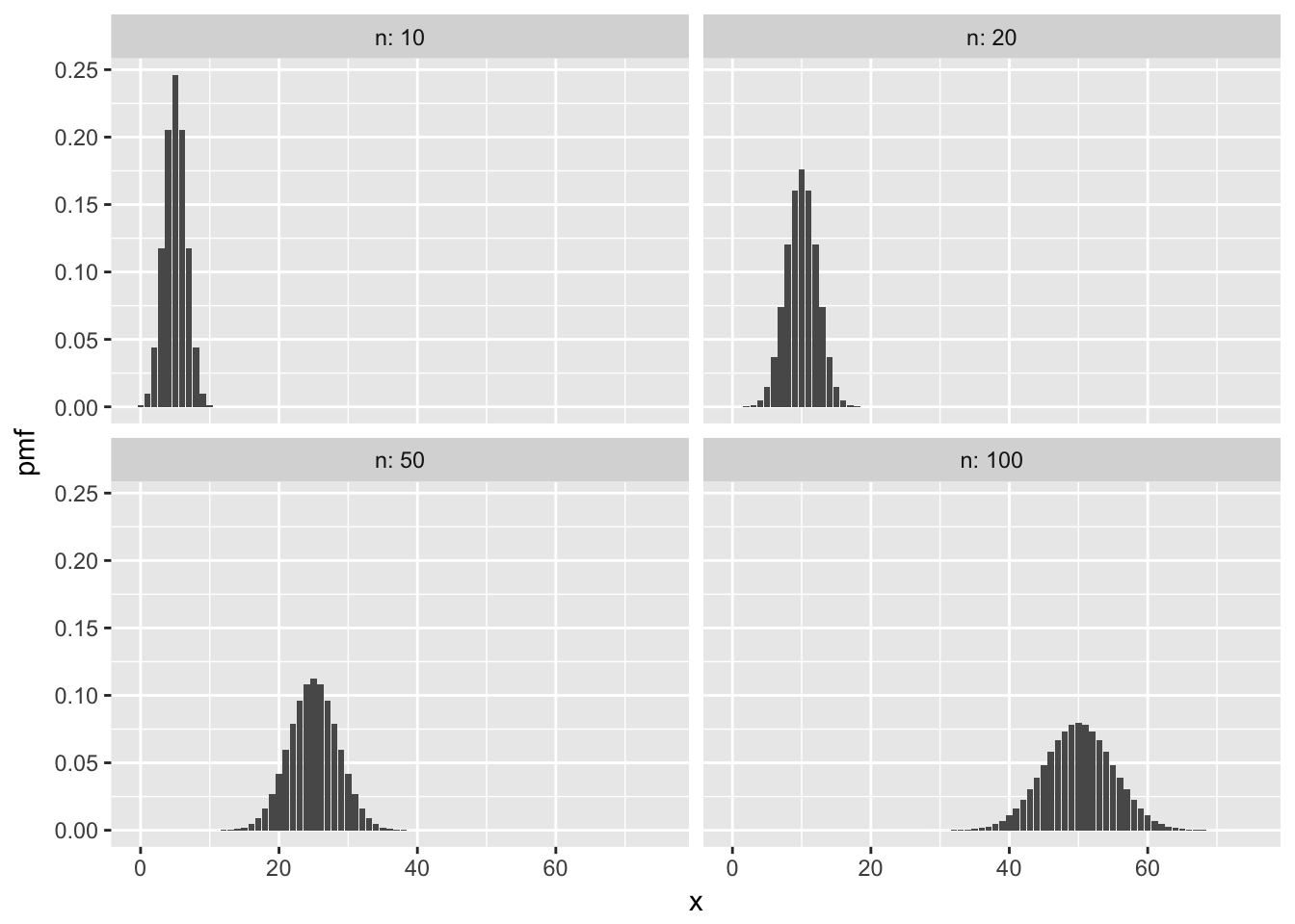
Here are some sample plots of the pmf of a binomial rv for various values of $n$ and $p= .5$².

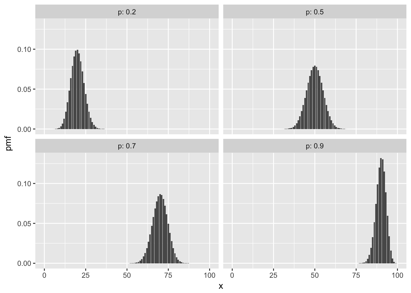
Here are some with $n = 100$ and various $p$.

3.4.2 Geometric Random Variable

Definition 3.3 A geometric random variable counts the number of failures in Bernoulli trials until the first success occurs.

A geometric random variable can take on values $0,1,2,\dotsc$. The pmf of a geometric rv is given by \[ p(x) = p(1-p)^{x} \qquad x = 0,\ldots \] Note that $\sum_x p(x) = 1$ by the sum of a geometric series formula.

Theorem 3.5 Let $X$ be a geometric random variable with probability of success $p$. Then

The expected value of $X$ is $\frac{(1-p)}{p}$.
The variance of $X$ is $\frac{(1-p)}{p^2}$

Example A die is tossed until the first 6 occurs. What is the probability that it takes 4 or more tosses? We let $X$ be a geometric random variable with probability of success $1/6.$ Since $X$ counts the number of failures before the first success, the problem is asking us to compute \[ P(X \ge 3) = \sum_{j=3}^\infty P(X = j) \] One approach is to approximate the infinite sum of the pdf dgeom:

sum(dgeom(3:1000, 1/6))

## [1] 0.5787037

Better is to use the built-in cdf function pgeom:

pgeom(2, 1/6, lower.tail = FALSE)

## [1] 0.5787037

Setting lower.tail = FALSE forces R to compute $P(X > 2) = P(X \ge 3)$ since $X$ is discrete.

Another approach is to apply rules of probability: $P(X \ge 3) = 1 - P(X < 3) = 1 - P(X \le 2)$. Then with R:

1 - pgeom(2,1/6)

## [1] 0.5787037

1 - sum(dgeom(0:2, 1/6))

## [1] 0.5787037

All of these show there is about a 0.58 probability that it will take four or more tosses to roll a six. Does this sound reasonable? The expected number of tosses (failures) before one obtains a 6 is $\frac{1-p}{p} = \frac{5/6}{1/6} = 5$, so $P(X \ge 3) \approx 0.58$ is not surprising at all.

The standard deviation of the number of tosses is $\sqrt{\frac{5/6}{1/6^2}} = \sqrt{30} \approx 5.5$. Using the rule of thumb that “most” data lies within two standard deviations of the mean, we would be surprised (but perhaps not shocked) if it took more than $5 + 2\sqrt(30) \approx 16$ rolls before we finally rolled a 6. The probability of it taking more than 16 rolls is $P(X \ge 16) \approx .054$.

3.4.2.1 Proof that the mean of a geometric rv is $\frac{1-p}{p}$ (Optional)

Let $X$ be a geometric rv with probability of success $p$. We show that $E[X] = \frac{1-p}{p}$. We must compute \[ E[X] = \sum_{x = 0}^\infty x p(1 - p)^x = (1 - p)p \sum_{x=1}^\infty x(1-p)^{x-1} \] Let $q = 1- p$ and see \[\begin{align*} E[X] &= q( 1-q) \sum_{x=1}^\infty xq^{x-1} = q(1 - q) \sum_{x=1}^\infty \frac {d}{dq} q^x \\ &= q(1 - q) \frac {d}{dq} \sum_{x=1}^\infty q^x = q(1- q) \frac{d}{dq} (1 - q)^{-1} = \frac{q(1-q)}{(1- q)^2}\\ &=\frac{q}{1-q} = \frac{1-p}{p} \end{align*}\]

For the variance, the interested reader can compute $E[X^2]$ using $E[X^2] = E[X(X - 1)] + E[X]$ and a similar method as that which was used in the above computation.

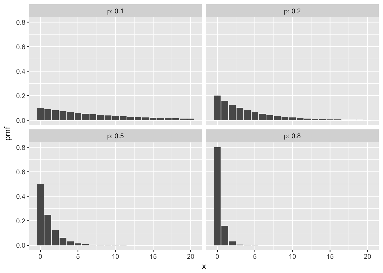
Here are some plots of pmfs with various $p$.

3.4.3 Poisson Random Variables

This section discusses the Poisson random variable, which comes from a Poisson process. Suppose events occur spread over time span $[0,T]$. If the occurrences of the event satisfy the following properties, then the events form a Poisson process:

The probability of an event occurring in a time interval $[a,b]$ depends only on the length of the interval $[a,b]$.
If $[a,b]$ and $[c,d]$ are disjoint time intervals, then the probability that an event occurs in $[a,b]$ is independent of whether an event occurs in $[c,d]$. (That is, knowing that an event occurred in $[a,b]$ does not change the probability that an event occurs in $[c,d]$.)
Two events cannot happen at the same time. (Formally, we need to say something about the probability that two or more events happens in the interval $[a, a + h]$ as $h\to 0$.)
The probability of an event occuring in a time interval $[a,a + h]$ is roughly $\lambda h$, for some constant $\lambda$.

Property (4) says that events occur at a certain rate, which is denoted by $\lambda$.

Definition 3.4 A Poisson random variable with rate $\lambda$ counts the number of events that occur in the Poisson process.

The pmf of $X$ when $X$ is Poisson with rate $\lambda$ is \[ p(x) = \frac 1{x!} \lambda^x e^{-\lambda}, \qquad x = 0,1,\ldots \] Note that the Taylor series for $e^t$ is $\sum_{n=0}^\infty \frac 1{n!} t^n$, which can be used to show that $\sum_x p(x) = 1$.

Theorem 3.6 The mean and variance of a Poisson random variable are both $\lambda$.

Example

Suppose a typist makes typos at a rate of 3 typos per page. What is the probability that they will make exactly 5 typos on a two page sample?

Here, we assume that typos follow the properties of a Poisson rv. It is not clear that they follow it exactly. For example, if the typist has just made a mistake, it is possible that their fingers are no longer on home position, which means another mistake is likely, violating the independence rule (2). Nevertheless, assuming the typos are Poisson is a reasonable approximation.

The rate at which typos occur per two pages is 6, so we use $\lambda = 6$ in the formula for Poisson. We get \[ P(X = 5) = \frac{6^5}{5!} e^{-6} \approx 0.16. \] Using R, and the pdf dpois:

dpois(5,6)

## [1] 0.1606231

There is a 0.16 probability of making exactly five typos on a two-page sample.

Often, when modeling a count of something, you need to choose between binomial, geometric, and Poisson. The binomial and geometric random variables both come from Bernoulli trials, where there is a sequence of individual trials each resulting in success or failure. In the Poisson process, events are spread over a time interval, and appear at random.

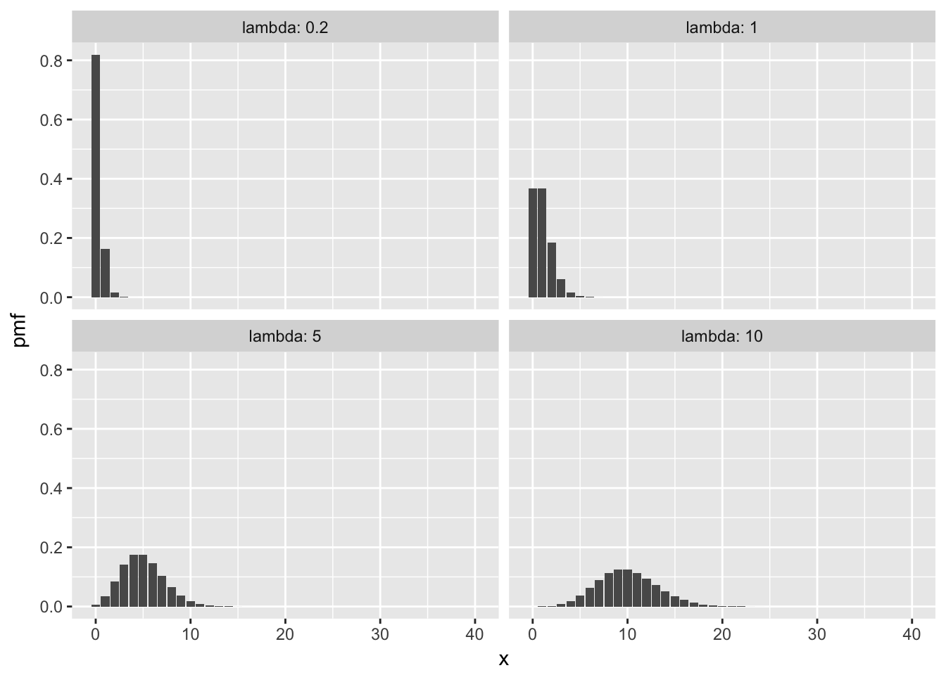
Here some plots of pmfs with various means.

3.4.4 Negative Binomial (Optional)

Example Suppose you repeatedly roll a fair die. What is the probability of getting exactly 14 non-sixes before getting your second 6?

As you can see, this is an example of repeated Bernoulli trials with $p = 1/6$, but it isn’t exactly geometric because we are waiting for the second success. This is an example of a negative binomial random variable.

More generally, suppose that we observe a sequence of Bernoulli trials with probability of success prob. If $X$ denotes the number of failures x before the nth success, then $X$ is a negative binomial random variable with parameters n and p. The probability mass function of $X$ is given by

\[ p(x) = {{x + n - 1}\choose{x}} p^n (1 - p)^x, \qquad x = 0,1,2\ldots \]

The mean of a negative binomial is $n p/(1 - p)$, and the variance is $n p /(1 - p)^2$. The root R function to use with negative binomials is nbinom, so dnbinom is how we can compute values in R. The function dnbinom uses prob for $p$ and size for $n$ in our formula. So, to continue with the example above, the probability of obtaining exactly 14 non-sixes before obtaining 2 sixes is:

dnbinom(x = 14, size = 2, prob = 1/6)

## [1] 0.03245274

Note that when size = 1, negative binomial is exactly a geometric random variable, e.g.

dnbinom(x = 14, size = 1, prob = 1/6)

## [1] 0.01298109

dgeom(14, prob = 1/6)

## [1] 0.01298109

3.4.5 Hypergeometric (Optional)

Consider the experiment which consists of sampling without replacement from a population that is partitioned into two subgroups - one subgroup is labeled a “success” and one subgroup is labeled a “failure”. The random variable that counts the number of successes in the sample is an example of a hypergeometric random variable.

To make things concrete, we suppose that we have $m$ successes and $n$ failures. We take a sample of size $k$ (without replacement) and we let $X$ denote the number of successes. Then \[ P(X = x) = \frac{{m \choose x} { n \choose {k - x}} }{{m + n} \choose k} \] We also have \[ E[X] = k (\frac{m}{m + n}) \] which is easy to remember because $k$ is the number of samples taken, and the probability of a success on any one sample (with no knowledge of the other samples) is $\frac {m}{m + n}$. The variance is similar to the variance of a binomial as well, \[ V(X) = k \frac{m}{m+n} \frac {n}{m+n} \frac {m + n - k}{m + n - 1} \] but we have the “fudge factor” of $ $, which means the variance of a hypergeometric is less than that of a binomial. In particular, when $m + n = k$, the variance of $X$ is 0. Why?

When $m + n$ is much larger than $k$, we will approximate a hypergeometric random variable with a binomial random variable with parameters $n = m + n$ and $p = \frac {m}{m + n}$. Finally, the R root for hypergeometric computations is hyper. In particular, we have the following example:

Example 15 US citizens and 20 non-US citizens pass through a security line at an airport. Ten are randomly selected for further screening. What is the probability that 2 or fewer of the selected passengers are US citizens?

In this case, $m = 15$, $n = 20$, and $k = 10$. We are looking for $P(X \le 2)$, so

sum(dhyper(x = 0:2, m = 15, n = 20, k = 10))

## [1] 0.08677992

3.5 Special Continuous Random Variables

In this section, we discuss the uniform, exponential, and normal random variables. There are many others that are useful, and we will cover them as needed in the rest of the text.

3.5.1 Uniform Random Variable

A uniform random $X$ over the interval $(a,b)$ satisfies the property that for any interval inside of $(a,b)$, the probability that $X$ is in that interval depends only on the length of the interval. The pdf is given by \[ f(x) = \begin{cases} \frac{1}{b -a} & a \le x \le b\\0&{\rm otherwise} \end{cases} \] The expected value of $X$ is $\int_a^b \frac x{b - a} \, dx = \frac{b + a}2$, and the variance is $\sigma^2 = \frac{b^2 - a^2}{12}$.

Example A random number is chosen between 0 and 10. What is the probability that it is bigger than 7, given that it is bigger than 6?

\[ P(X > 7\ |\ X > 6) = \frac{P(X > 7 \cap X > 6)}{P(X > 6)} = \frac{P(X > 7)}{P(X > 6)} =\frac{3/10}{4/10} = \frac{3}{4}. \]

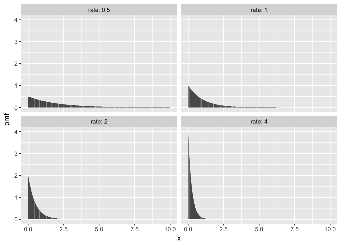
3.5.2 Exponential Random Variable

An exponential random variable $X$ with rate $\lambda$ has pdf \[ f(x) = \lambda e^{-\lambda x}, \qquad x > 0 \] Exponential rv’s are useful for, among other things, modeling the waiting time until the first occurrence in a Poisson process. So, the waiting time until an electronic component fails, or until a customer enters a store could be modeled by exponential random variables.

The mean of an exponential random variable is $\mu = 1/\lambda$ and the variance is $\sigma^2 = 1/\lambda^2$.

Here are some plots of pdf’s with various rates.

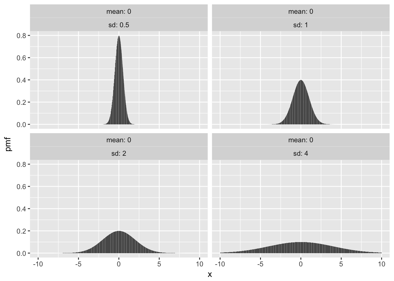
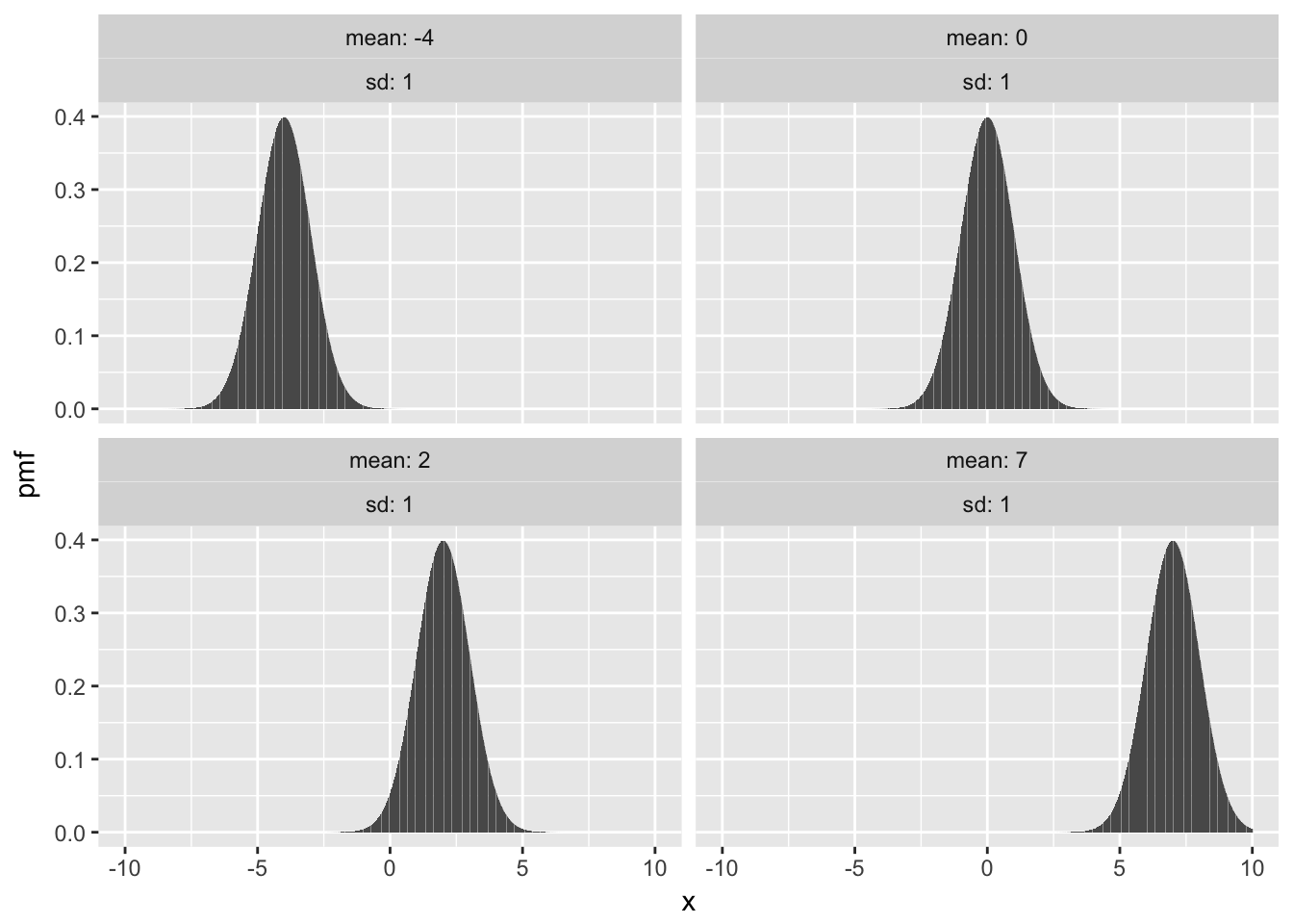
3.5.3 Normal Random Variable

A normal random variable with mean $\mu$ and standard deviation $\sigma$ has pdf given by \[ f(x) = \frac 1{\sigma\sqrt{2\pi}} e^{-(x - \mu)^2/(2\sigma^2)} \] The mean of a normal rv is $\mu$ and the standard deviation is $\sigma$. We will see many uses for normal random variables throughout the book, but for now let’s just compute some probabilities when $X \sim {\rm Normal}(\mu = 2, \sigma = 2)$.

$P(X \le 4)$ = pnorm(4,mean = 2,sd = 4)
$P(0 \le X \le 2)$ = pnorm(2,2,4) - pnorm(0,2,4).
Find the value of $q$ such that $P(X \le q) = .75$. $q$ = qnorm(.75,2,4). We get about 4.7; we can check it with pnorm(4.7,2,4).

Here are some plots with fixed mean 0 and various sd, followed by fixed sd and various means.

3.6 Independent Random Variables

We say that two random variables, $X$ and $Y$, are independent if knowledge of the outcome of $X$ does not give probabilistic information about the outcome of $Y$ and vice versa. As an example, let $X$ be the amount of rain (in inches) recorded at Lambert Airport on a randomly selected day in 2017, and let $Y$ be the height of a randomly selected person in Botswana. It is difficult to imagine that knowing the value of one of these random variables could give information about the other one, and it is reasonable to assume that the rvs are independent. On the other hand, if $X$ and $Y$ are the height and weight of a randomly selected person in Botswana, then knowledge of one variable could well give probabilistic information about the other. For example, if you know a person is 70 inches tall, it is very unlikely that they weigh 12 pounds.

We would like to formalize that notion by saying that whenever $E, F$ are subsets of ${\mathbb R}$, $P(X\in E|Y\in F) = P(X \in E)$. There are several issues with formalizing the notion of independence that way, so we give a definition that is somewhat further removed from the intuition.

The random variables $X$ and $Y$ are independent if

For all $x$ and $y$, $P(X = x, Y = y) = P(X = x) P(Y = y)$ if $X$ and $Y$ are discrete.
For all $x$ and $y$, $P(X \le x, Y \le Y) = P(X \le x) P(Y \le y)$ if $X$ and $Y$ are continuous.

For our purposes, we will often be assuming that random variables are independent.

3.7 Using R to compute probabilities

For all of the random variables that we have mentioned so far (and many more!), R has built in capabilities of computing probabilities. The syntax is broken down into two pieces: the root and the prefix. The root determines which random variable that we are talking about, and here are the names of the ones that we have covered so far:

binom is binomial
geom is geometric
pois is Poisson
unif is uniform
exp is exponential
norm is normal

The available prefixes are

p computes the cumulative distribution
d computes pdf or pmf
r samples from the rv
q quantile function

For now, we will focus on the prefixes p and d.

Example Let $X$ be binomial with $n = 10$ and $p = .3$.

Compute $P(X = 5)$.

We are interested in the pmf of a binomial rv, so we will use the R command dbinom as follows:

dbinom(5, 10, .3)

## [1] 0.1029193

and we see that answer is about 1/10.

Compute $P(1 \le X \le 5)$.

We want to sum $P(X = 1) + P(X = 2) + P(X = 3) + P(X = 4) + P(X = 5)$. We could do that the long way as follows:

dbinom(5, 10, .3) + dbinom(4, 10, .3) + dbinom(3, 10, .3) + dbinom(2, 10, .3) + dbinom(1, 10, .3)

## [1] 0.9244035

But, that is going to get old very quickly. Note that dbinom also allows vectors as arguments, so we can compute all of the needed probabilities like this:

dbinom(1:5, 10, .3)

## [1] 0.1210608 0.2334744 0.2668279 0.2001209 0.1029193

And, all we need to do is add those up:

sum(dbinom(1:5, 10 , .3))

## [1] 0.9244035

Check that we got the same answer. Yep.

Example Let $X$ be a normal random variable with mean 1 and standard deviation 5.

Compute $P(X \le 1)$.

It is not easy to use the same technique as before, because we would need to compute \[ \int_{-\infty}^1 {\text {dnorm(x,1,5))}} \, dx \] But, note that the probability we are trying to compute is exactly the cdf, so we want to use pnorm.

pnorm(1,1,5)

## [1] 0.5

Compute $P(1 \le X \le 5)$.

Here, we compute the probability that $X$ is less than or equal to five, and subtract the probability that $X$ is less than 1. Since $X$ is continuous, that is the same as computing \[ P(X \le 5) - P(X \le 1) \]

pnorm(5,1,5) - pnorm(1,1,5)

## [1] 0.2881446

Note to use p + a discrete rv, you will need to make adjustments to the above technique, e.g. if $X$ is binomial(10, .3) and you want to compute $P(1\le X \le 5)$, you would use

pbinom(5,10,.3) - pbinom(0,10,.3)

## [1] 0.9244035

3.8 A ggplot interlude

In this short section, we introduce the basics of plotting using ggplot. We will go into more details later, but for now, we want to know how to plot scatterplots and lines using ggplot.

The package ggplot2 is not part of the base R package, and needs to be installed on your machine. If it has not already been installed, then you need to do so (you can use the Install button under the Packages tab in RStudio, or see this) and use the command library(ggplot2) to be able to use it.

If you have never used ggplot before, it works differently than other graphing utilities that I have seen. The basic idea is that the call of ggplot() sets up the default data that will be plotted and the basic aesthetic mappings. For our purposes in this section, the first argument of ggplot will be a data frame that we wish to visualize, and the second argument will be aes(x = , y = ). You will need to tell ggplot which variable you want to be considering as the independent variable (x) and which is the dependent variable (y).

For example, consider the mtcars data set. If we wish to plot mpg versus disp, we would start by typing ggplot(mtcars, aes(x = disp, y = mpg)). Run this now. As you can see, ggplot has set up the axes according to disp and mpg with reasonable values, but no data has been plotted. This is because we haven’t told ggplot what we want to do with the data. Do we want a histogram? A scatterplot? A heatmap? Well, let’s assume we want a scatterplot here. We need to add the scatterplot to the pre-existing plot. We do that as follows:

library(ggplot2) #Only need to do once
ggplot(mtcars, aes(x = disp, y = mpg)) +
  geom_point()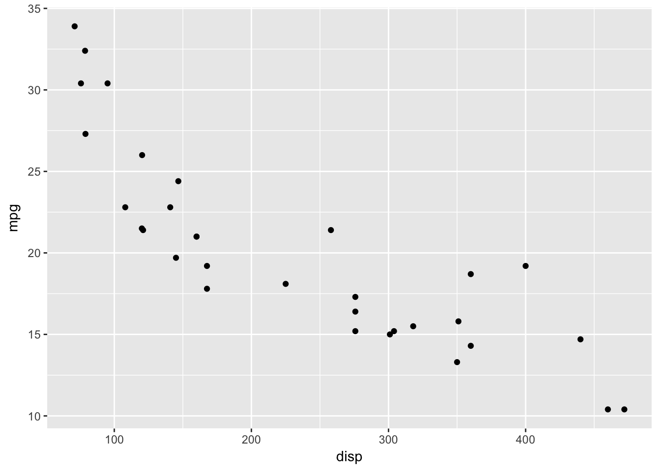

Later, we will see that geom_point() has its own aesthetic mappings and options, and we can combine things in more complicated and beautiful ways. But for now, we just want the basic scatterplot.

In order to graph a function, we would create a data frame with the $x$ values and $y$ values that we wish to plot, and use geom_line(), as follows.

Example Plot the pdf of a normal rv with mean 1 and standard deviation 2.

xvals <- seq(-4,6,.01)
plotdata <- data.frame(x = xvals, y = dnorm(xvals, 1, 2))
ggplot(plotdata, aes(x = x, y = y)) +
  geom_line()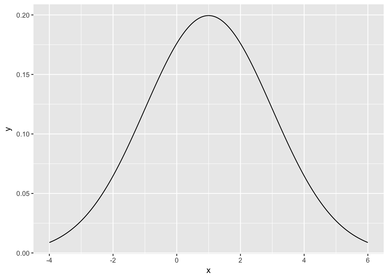

Example Plot the pmf of a geometric random variable with probability of success $1/3$.

xvals <- 0:20
plotdata <- data.frame(x = xvals, y = dgeom(xvals, 1/3))
ggplot(plotdata, aes(x, y)) + geom_bar(stat = "identity")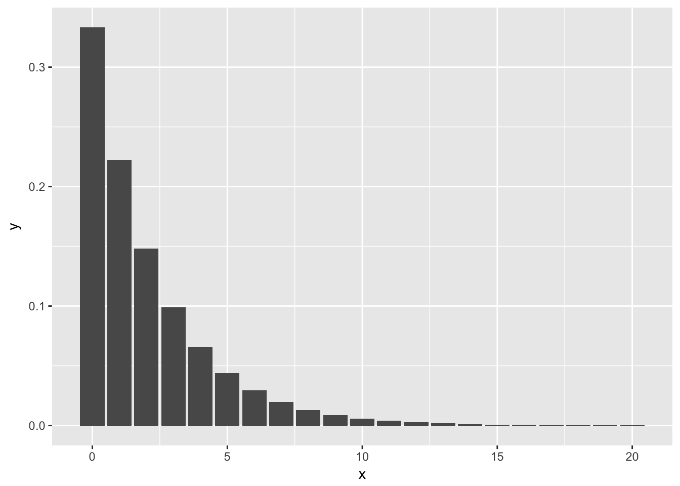

The reason we have to add stat = "identity" to the above plot is that geom_bar() normally plots the number of observances of the x-values versus the x-values. In this case, however, we already have the y-values that we want plotted. We are using geom_bar() just to get the form of the graph to look like this, so we tell geom_bar() to use the y-values in the aesthetic mapping by including stat = "identity".

3.9 Summary

Here is a list of the (non-optional) random variables that we introduced in this section, together with pmf/pdf, expected value, variance and root R function.

RV	PMF/PDF	Range	Mean	Variance	R Root
Binomial	${{n}\choose {x}} p^x(1 - p)^{n - x}$	$0\le x \le n$	$np$	$np(1 - p)$	`binom`
Geometric	$p(1-p)^{x}$	$x \ge 0$	$\frac{1-p}{p}$	$\frac{1-p}{p^2}$	`geom`
Poisson	$\frac {1}{x!} \lambda^x e^{-\lambda}$	$x \ge 0$	$\lambda$	$\lambda$	`pois`
Uniform	$\frac{1}{b - a}$	$a \le x \le b$	$\frac{a + b}{2}$	$\frac{b^2 - a^2}{12}$	`unif`
Exponential	$\lambda e^{-\lambda x}$	$x \ge 0$	$1/\lambda$	$1/\lambda^2$	`exp`
Normal	$\frac 1{\sigma\sqrt{2\pi}} e^{(x - \mu)^2/(2\sigma^2)}$	$-\infty < x < \infty$	$\mu$	$\sigma^2$	`norm`

3.10 Exercises

Let $X$ be a discrete random variable with probability mass function given by \[ p(x) = \begin{cases} 1/4 & x = 0 \\ 1/2 & x = 1\\ 1/8 & x = 2\\ 1/8 & x = 3 \end{cases} \]
1. Verify that $p$ is a valid probability mass function.
2. Find the mean and variance of $X$.
3. Find $P(X \ge 2)$.
4. Find $P(X \ge 2\ |\ X \ge 1)$.
Plot the pdf and cdf of a uniform random variable on the interval $[0,1]$.
Compare the cdf and pdf of an exponential random variable with rate $\lambda = 2$ with the cdf of an exponential rv with rate 1/2. (If you wish to read ahead in the section on plotting, you can learn how to put both plots on the same axes, with different colors.)
Compare the pdfs of three normal random variables, one with mean 1 and standard deviation 1, one with mean 1 and standard deviation 10, and one with mean -4 and standard deviation 1.
Let $X$ be a normal rv with mean 1 and standard deviation 2.
1. Find $P(a \le X \le a + 2)$ when $a = 3$.
2. Sketch the graph of the pdf of $X$, and indicate the region that corresponds to your answer in the previous part.
3. Find the value of $a$ such that $P(a \le X \le a + 2)$ is the largest.
Let $X$ be an exponential rv with rate $\lambda = 1/4$.
1. What is the mean of $X$?
2. Find the value of $a$ such that $P(a \le X \le a + 1)$ is maximized. Is the mean contained in the interval $[a, a+1]$?
Let $X$ be a random variable with pdf $f(x) = 3(1 - x)^2$ when $0\le x \le 1$, and $f(x) = 0$ otherwise.
1. Verify that $f$ is a valid pdf.
2. Find the mean and variance of $X$.
3. Find $P(X \ge 1/2)$.
4. Find $P(X \ge 1/2\ |\ X \ge 1/4)$.
Is there a function which is both a valid pdf and a valid cdf? If so, give an example. If not, explain why not.
(Memoryless Property) Let $X$ be an exponential random variable with rate $\lambda$. If $a$ and $b$ are positive numbers, then \[ P(X > a + b\ |\ X > b) = P(X > a) \]
1. Explain why this is called the memoryless property.
2. Show that for an exponential rv $X$ with rate $\lambda$, $P(X > a) = e^{-a\lambda}$.
3. Use the result in (b) to prove the memoryless property for exponential random variables.
Let $X$ be a Poisson rv with mean 3.9.
1. Create a plot of the pmf of $X$.
2. What is the most likely outcome of $X$?
3. Find $a$ such that $P(a \le X \le a + 1)$ is maximized.
4. Find $b$ such that $P(b \le X \le b + 2)$ is maximized.
For each of the following descriptions of a random variable, indicate whether it can best be modeled by binomial, geometric, Poisson, uniform, exponential or normal. Answer the associated questions. Note that not all of the experiments yield rv’s that are exactly of the type listed above, but we are asking about reasonable modeling.
1. Let $Y$ be the random variable that counts the number of sixes which occur when a die is tossed 10 times. What type of random variable is $Y$? What is $P(Y=3)$? What is the expected number of sixes? What is ${\rm Var}(Y)$?
2. Let $U$ be the random variable which counts the number of accidents which occur at an intersection in one week. What type of random variable is $U$? Suppose that, on average, 2 accidents occur per week. Find $P(U=2)$, $E(U)$ and ${\rm Var}(U)$.
3. Suppose a stop light has a red light that lasts for 60 seconds, a green light that lasts for 30 seconds and a yellow light that lasts for 5 seconds. When you first observe the stop light, it is red. Let $X$ denote the time until the light turns green. What type of rv would be used to model $X$? What is its mean?
4. Customers arrive at a teller’s window at a uniform rate of 5 per hour. Let $X$ be the length in minutes of time that the teller has to wait until they see their first customer after starting their shift. What type of rv is $X$? What is its mean? Find the probability that the teller waits less than 10 minutes for their first customer.
5. A coin is tossed until a head is observed. Let $X$ denote the total number of tails observed during the experiment. What type of rv is $X$? What is its mean? Find $P(X \le 3)$.
6. Let $X$ be the recorded body temperature of a healthy adult in degrees Fahrenheit. What type of rv is $X$? Estimate its mean and standard deviation, based on your knowledge of body temperatures.
Suppose you turn on a soccer game and see that the score is 1-0 after 30 minutes of play. Let $X$ denote the time (in minutes from the start of the game) that the goal was scored. What type of rv is $X$? What is its mean?
(Requires optional sections) Prove that the mean of a Poisson rv with parameter $\lambda$ is $\lambda$.
Roll two ordinary dice and let $X$ be their sum. Draw the pmf and cmf for X. Compute the mean and standard deviation of $X$.
Suppose you roll two ordinary dice. Calculate the expected value of their product.
Go to the Missouri lottery Pick 3 web page http://www.molottery.com/pick3/pick3.jsp and compute the expected value of these bets:
1. $1 Front Pair
2. $1 Back Pair
3. $6 6-way combo
4. $3 3-way combo
5. $1 1-off
Suppose you take a 20 question multiple choice test, where each question has four choices. You guess randomly on each question. What is your expected score? What is the probability you get 10 or more questions correct?
Steph Curry is a 91% free throw shooter. Suppose he shoots 10 free throws in a game. What is his expected number of shots made? What is the probability that he makes at least 8 free throws?
Suppose that 55% of voters support Proposition A.
1. You poll 200 voters. What is the expected number that support the measure?
2. What is the margin of error for your poll (two standard deviations)?
3. What is the probability that your poll claims that Proposition A will fail?
4. How large a poll would you need to reduce your margin of error to 2%?
The charge $e$ on one electron is too small to measure. However, one can make measurements of the current $I$ passing through a detector. If $N$ is the number of electrons passing through the detector in one second, then $I = eN$. Assume $N$ is Poisson. Show that the charge on one electron is given by $\frac{{\rm Var}(I)}{E(I)}$.
Climbing rope will break if pulled hard enough. Experiments show that 10.5mm Dynamic nylon rope has a mean breaking point of 5036 lbs with a standard deviation of 122 lbs. Assume breaking points of rope are normally distributed.
1. Sketch the distribution of breaking points for this rope.
2. What proportion of ropes will break with 5000 lbs of load?
3. At what load will 95% of all ropes break?
There exist naturally occurring random variables that are neither discrete nor continuous. Suppose a group of people is waiting for one more person to arrive before starting a meeting. Suppose that the arrival time of the person is exponential with mean 4 minutes, and that the meeting will start either when the person arrives, or after 5 minutes, whichever comes first. Let $X$ denote the length of time the group waits before starting the meeting.
1. Find $P(0 \le X \le 4)$.
2. Find $P(X = 5)$.
A roulette wheel has 38 slots and a ball that rolls until it falls into one of the slots, all of which are equally likely. Eighteen slots are black numbers, eighteen are red numbers, and two are green zeros. If you bet on “red”, and the ball lands in a red slot, the casino pays you your bet, otherwise the casino wins your bet.
1. What is the expected value of a $1 bet on red?
2. Suppose you bet $1 on red, and if you win you “let it ride” and bet $2 on red. What is the expected value of this plan?
One (questionable) roulette strategy is called bet doubling. You bet $1 on red, and if you win, you pocket the $1. If you lose, you double your bet so you are now betting $2 on red, but have lost $1. If you win, you win $2 for a $1 profit, which you pocket. If you lose again, you double your bet to $4 (having already lost $3). Again, if you win, you have $1 profit, and if you lose, you double your bet again. This guarantees you will win $1, unless you run out of money to keep doubling your bet.
1. Say you start with a bankroll of $127. How many bets can you lose in a row without losing your bankroll?
2. If you have a $127 bankroll, what is the probability that bet doubling wins you $1?
3. What is the expected value of the bet doubling strategy with a $127 bankroll?
4. If you play the bet doubling strategy with a $127 bankroll, how many times can you expect to play before you lose your bankroll?

That is, the variance is greater than or equal to zero.↩
You don’t need to know the R code to generate this yet, but here it is: library(dplyr) library(ggplot2) binomdata <- data.frame(x = rep(0:75, 4)) binomdata <- mutate(binomdata, n = c(rep(10, 76),rep(20,76),rep(50,76),rep(100,76)), pmf = dbinom(x,n,p=.5)) ggplot(binomdata, aes(x = x, y = pmf)) + geom_bar(stat = "identity") + facet_wrap(~n, labeller = "label_both")↩

RV	PMF/PDF	Range	Mean	Variance	R Root
Binomial	\({{n}\choose {x}} p^x(1 - p)^{n - x}\)	\(0\le x \le n\)	\(np\)	\(np(1 - p)\)	`binom`
Geometric	\(p(1-p)^{x}\)	\(x \ge 0\)	\(\frac{1-p}{p}\)	\(\frac{1-p}{p^2}\)	`geom`
Poisson	\(\frac {1}{x!} \lambda^x e^{-\lambda}\)	\(x \ge 0\)	\(\lambda\)	\(\lambda\)	`pois`
Uniform	\(\frac{1}{b - a}\)	\(a \le x \le b\)	\(\frac{a + b}{2}\)	\(\frac{b^2 - a^2}{12}\)	`unif`
Exponential	\(\lambda e^{-\lambda x}\)	\(x \ge 0\)	\(1/\lambda\)	\(1/\lambda^2\)	`exp`
Normal	\(\frac 1{\sigma\sqrt{2\pi}} e^{(x - \mu)^2/(2\sigma^2)}\)	\(-\infty < x < \infty\)	\(\mu\)	\(\sigma^2\)	`norm`

Foundations of Statistics with R