4 Simulation of Random Variables
In this chapter we discuss simulation related to random variables. We will simulate probabilities related to random variables, and more importantly for our purposes, we will simulate pdfs and pmfs of random variables.
4.1 Estimating probabilities of rvs via simulation.
In order to run simulations with random variables, we will use the R command r + distname, where distname is the name of the distribution, such as unif, geom, pois, norm, exp or binom. The first argument to any of these functions is the number of samples to create.
Most distname choices can take additional arguments that affect their behavior. For example, if I want to create a random sample of size 100 from a normal random variable with mean 5 and sd 2, I would use rnorm(100,5,2). Without the additional arguments, rnorm gives the standard normal random variable, with mean 0 and sd 1. For example, rnorm(10000) gives 10000 random values of the standard normal random variable \(Z\).
Example Let \(Z\) be a standard normal random variable. Estimate \(P(Z > 1)\).
z <- rnorm(10000)
mean(z > 1)
## [1] 0.15561 - pnorm(1)## [1] 0.1586553Example Let \(Z\) be a standard normal rv. Estimate \(P(Z^2 > 1)\).
z <- rnorm(10000)
mean(z^2 < 1)
## [1] 0.6822Example Estimate the mean and standard deviation of \(Z^2\).
z <- rnorm(10000)
mean(z^2)
## [1] 0.9936186sd(z^2)## [1] 1.386947Example Let \(X\) and \(Y\) be independent standard normal random variables. Estimate \(P(XY > 1)\).
x <- rnorm(10000)
y <- rnorm(10000)
mean(x*y > 1)
## [1] 0.1062Note that this is not the same as the answer we got for \(P(Z^2 > 1)\).
4.2 Estimating discrete distributions
In this section, we show how to estimate via simulation the pmf of a discrete random variable. Let’s begin with an example.
Example Suppose that two dice are rolled, and their sum is denoted as \(X\). Estimate the pmf of \(X\) via simulation.
Recall that if we wanted to estimate the probability that \(X = 2\), for example, we would use
mean(replicate(10000, {dieRoll <- sample(1:6, 2, TRUE); sum(dieRoll) == 2}))## [1] 0.0268It is possible to repeat this replication for each value \(2,\ldots, 12\), but that would take a long time. More efficient is to keep track of all of the observations of the random variable, and divide each by the number of times the rv was observed. We will use table for this. Recall, table gives a vector of counts of each unique element in a vector. That is,
table(c(1,1,1,1,1,2,2,3,5,1))##
## 1 2 3 5
## 6 2 1 1indicates that there are 6 occurrences of “1”, 2 occurrences of “2”, and 1 occurrence each of “3” and “5”. To apply this to the die rolling, we create a vector of length 10,000 that has all of the observances of the rv \(X\), in the following way:
set.seed(1)
table(replicate(10000, {dieRoll <- sample(1:6, 2, TRUE); sum(dieRoll)}))
##
## 2 3 4 5 6 7 8 9 10 11 12
## 265 556 836 1147 1361 1688 1327 1122 853 581 264We then divide each by 10,000 to get the estimate of the pmf:
set.seed(1)
table(replicate(10000, {dieRoll <- sample(1:6, 2, TRUE); sum(dieRoll)}))/10000
##
## 2 3 4 5 6 7 8 9 10 11
## 0.0265 0.0556 0.0836 0.1147 0.1361 0.1688 0.1327 0.1122 0.0853 0.0581
## 12
## 0.0264And, there is our estimate of the pmf of \(X\). In particular, we estimate the probability of rolling an 11 to be 0.0581.
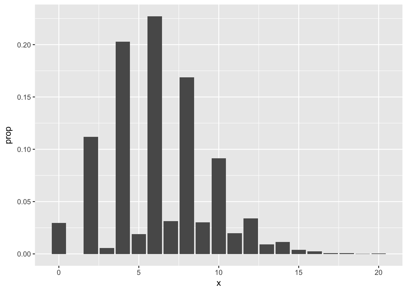
Example Suppose fifty randomly chosen people are in a room. Let \(X\) denote the number of people in the room who have the same birthday as someone else in the room. Estimate the pmf of \(X\).
We will simulate birthdays by taking a random sample from 1:365 and storing it in a vector. The tricky part is counting the number of elements in the vector that are repeated somewhere else in the vector. We will create a table and add up all of the values that are bigger than 1. Like this:
birthdays <- sample(1:365, 50, replace = TRUE)
table(birthdays)
## birthdays
## 9 20 26 28 33 38 42 43 44 54 55 57 64 74 77 99 110 112
## 1 1 1 1 1 1 1 1 1 1 1 1 1 1 1 1 1 1
## 113 114 116 127 140 144 147 148 165 168 169 171 175 184 193 233 239 240
## 2 1 1 1 1 1 1 1 1 1 1 1 1 1 1 1 1 1
## 249 257 268 272 274 280 289 295 303 304 328 354 362
## 1 1 1 1 1 1 1 1 1 1 1 1 1We look through the table and see that anywhere there is a number bigger than 1, there are that many people who share that birthday. To count the number of people who share a birthday with someone else:
sum(table(birthdays)[table(birthdays) > 1])## [1] 2Now, we put that inside replicate, just like in the previous example.
set.seed(1)
birthdayTable <- table(replicate(10000, {birthdays <- sample(1:365, 50, replace = TRUE); sum(table(birthdays)[table(birthdays) > 1]) }))/10000
birthdayTable
##
## 0 2 3 4 5 6 7 8 9 10
## 0.0297 0.1118 0.0056 0.2029 0.0190 0.2271 0.0312 0.1687 0.0301 0.0914
## 11 12 13 14 15 16 17 18 19 20
## 0.0198 0.0338 0.0092 0.0115 0.0038 0.0025 0.0007 0.0007 0.0001 0.0004Looking at the pmf, our best estimate is that the most likely outcome is that 6 people in the room share a birthday with someone else, followed closely by 4 and then 8. Note that it is impossible for exactly one person to share a birthday with someone else in the room! It would be preferable for several reasons to have the observation \(P(X = 1) = 0\) listed in the table above, but we leave that for another day. Plotting the pmf from the table output is a little more complicated than we need to get into right now (see Section 6.4), but here is a plot.3
Example (Optional) Suppose you have a bag full of marbles; 50 are red and 50 are blue. You are standing on a number line, and you draw a marble out of the bag. If you get red, you go left one unit. If you get blue, you go right one unit. You draw marbles up to 100 times, each time moving left or right one unit. Let \(X\) be the number of marbles drawn from the bag until you return to 0 for the first time. Estimate the pmf of \(X\).
movements <- sample(c(replicate(50,1),replicate(50,-1)), 100, FALSE)
movements[1:10]
## [1] -1 -1 1 1 1 -1 -1 1 1 1cumsum(movements)[1:10]## [1] -1 -2 -1 0 1 0 -1 0 1 2which(cumsum(movements) == 0)## [1] 4 6 8 82 98 100min(which(cumsum(movements) == 0))## [1] 4Now, we just need to table it like we did before.
table(replicate(10000, {movements <- sample(c(replicate(50,1),replicate(50,-1)), 100, FALSE); min(which(cumsum(movements) == 0)) }))/10000##
## 2 4 6 8 10 12 14 16 18 20
## 0.5120 0.1263 0.0637 0.0385 0.0270 0.0217 0.0194 0.0143 0.0140 0.0095
## 22 24 26 28 30 32 34 36 38 40
## 0.0094 0.0081 0.0066 0.0061 0.0073 0.0056 0.0053 0.0043 0.0031 0.0036
## 42 44 46 48 50 52 54 56 58 60
## 0.0036 0.0032 0.0032 0.0038 0.0027 0.0025 0.0025 0.0022 0.0029 0.0029
## 62 64 66 68 70 72 74 76 78 80
## 0.0027 0.0032 0.0025 0.0025 0.0025 0.0019 0.0031 0.0019 0.0031 0.0029
## 82 84 86 88 90 92 94 96 98 100
## 0.0026 0.0025 0.0030 0.0026 0.0028 0.0031 0.0038 0.0036 0.0049 0.00954.3 Estimating continuous distributions
In this section, we show how to estimate the pdf of a continuous rv via simulation. As opposed to the discrete case, we will not get an explicit formula for the pdf, but we will rather get a graph of it.
Example Estimate the pdf of \(2Z\) when \(Z\) is a standard normal random variable
Our strategy is to take a random sample of size 10,000 and use the R function geom_density inside of ggplot2 to estimate the pdf. As before, we build our sample of size 10,000 up as follows:
A single value sampled from standard normal rv:
z <- rnorm(1)We multiply it by 2 to get a single value sampled from \(2Z\).
2 * z## [1] -0.05017198Now create 10,000 values of \(2Z\):
zData <- 2 * rnorm(10000)We then use ggplot to estimate and plot the pdf of the data, after converting to a data frame:
ggplot(data.frame(zData), aes(x = zData)) + geom_density()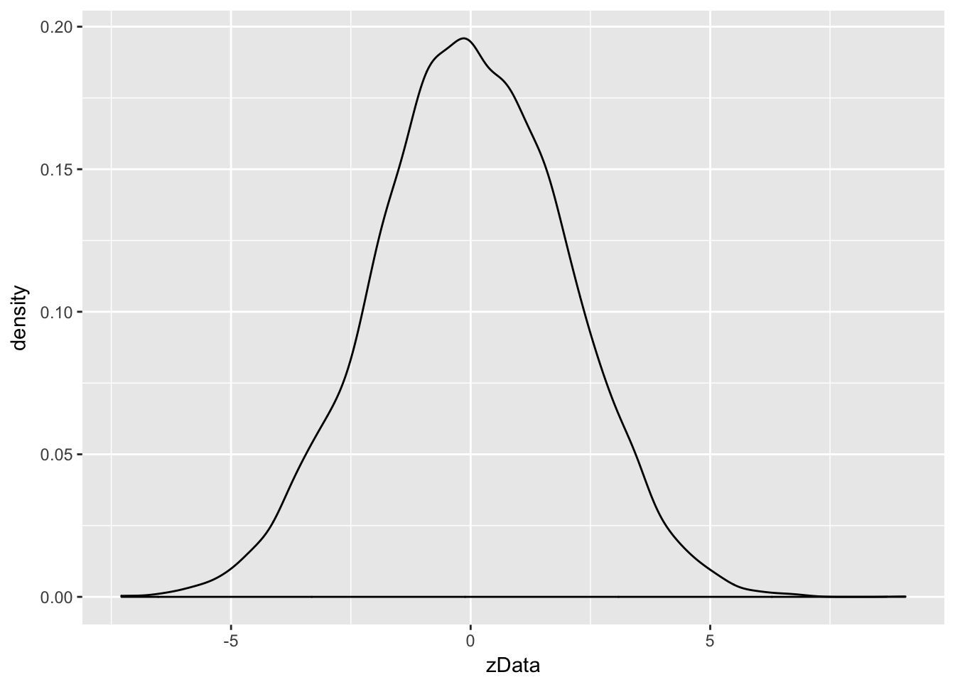
Notice that the most likely outcome of \(2Z\) seems to be centered around 0, just as it is for \(Z\), but that the spread of the distribution of \(2Z\) is twice as wide as the spread of \(Z\).
Example Estimate via simulation the pdf of \(\log\bigl(\left|Z\right|\bigr)\) when \(Z\) is standard normal.
expData <- log(abs(rnorm(10000)))
ggplot(data.frame(expData), aes(x = expData)) + geom_density()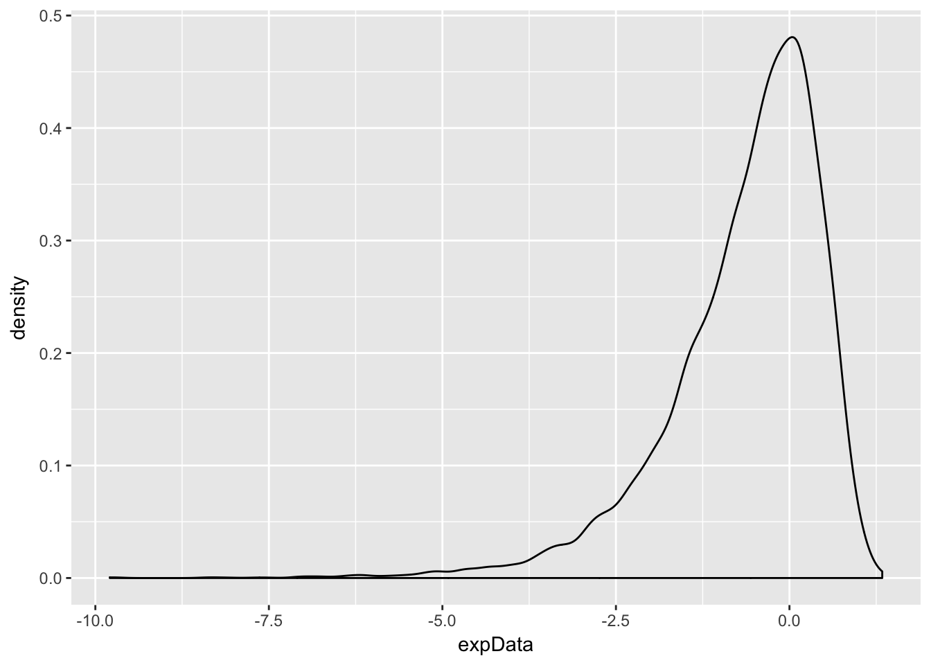
Both of the above worked pretty well, but there are issues when your pdf has discontinuities. Let’s see.
Example Estimate the pdf of \(X\) when \(X\) is uniform on the interval \([-1,1]\).
unifData <- runif(10000,-1,1)
ggplot(data.frame(unifData), aes(x = unifData)) + geom_density()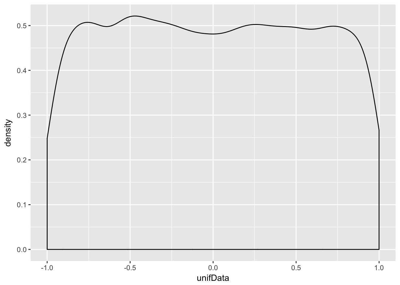
This distribution should be exactly 0.5 between -1 and 1, and zero everywhere else. The simulation is reasonable in the middle, but the discontinuities at the endpoints are not shown well. Increasing the number of data points helps, but does not fix the problem.
Example Estimate the pdf of \(X^2\) when \(X\) is uniform on the interval \([-1,1]\).
X2data <- runif(10000,-1,1)^2
ggplot(data.frame(X2data), aes(x = X2data)) + geom_density()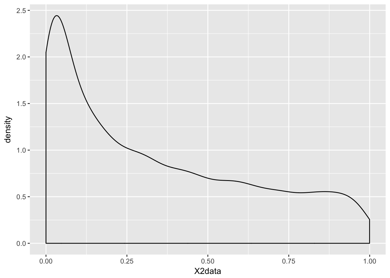
Example Estimate the pdf of \(X + Y\) when \(X\) and \(Y\) are exponential random variables with rate 2.
X <- rexp(10000,2)
Y <- rexp(10000,2)
sumData <- X + Y
ggplot(data.frame(sumData), aes(x = sumData)) + geom_density()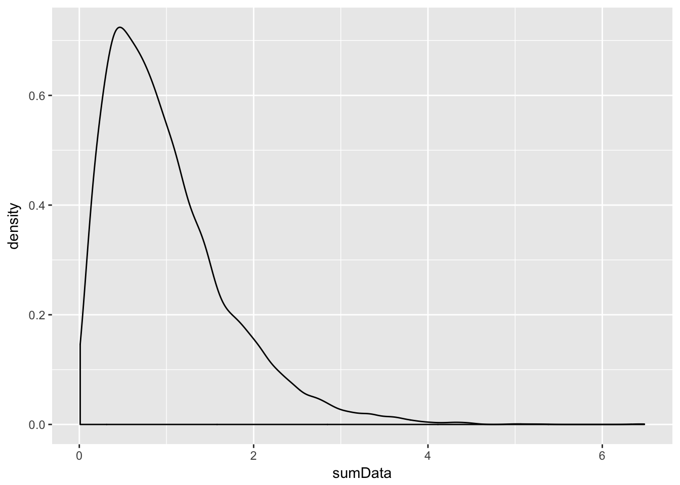
Example Estimate the density of \(X_1 + X_2 + \cdots + X_{20}\) when all of the \(X_i\) are exponential random variables with rate 2.
This one is trickier and the first one for which we need to use replicate to create the data. Let’s build up the experiment that we are replicating from the ground up.
Here’s the experiment of summing 20 exponential rvs with rate 2:
sum(rexp(20,2))## [1] 10.74181Now, we replicate it (10 times to test):
replicate(10, sum(rexp(20,2)))## [1] 11.046925 10.993640 11.597361 10.745458 10.653840 10.304673 11.596451
## [8] 14.613796 6.608730 9.030899Of course, we don’t want to just replicate it 10 times, we need about 10,000 data points to get a good density estimate.
sumExpData <- replicate(10000, sum(rexp(20,2)))
ggplot(data.frame(sumExpData), aes(x = sumExpData)) + geom_density()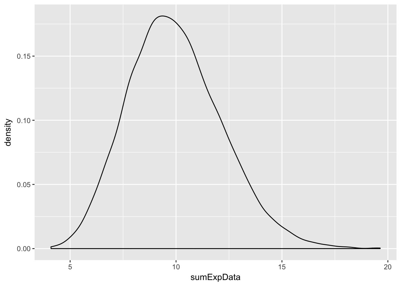
Note that this is starting to look like a normal random variable!!
4.4 Theorems about transformations of random variables
In this section, we will be estimating the pdf of transformations of random variables and comparing them to known pdfs. The goal will be to find a known pdf that closely matches our estimate, so that we can develop some theorems.
Example Compare the pdf of \(2Z\), where \(Z\sim \text{Normal}(0,1)\) to the pdf of a normal random variable with mean 0 and standard deviation 2.
We already saw how to estimate the pdf of \(2Z\), we just need to plot the pdf of \(\text{Normal}(0,2)\) on the same graph. The pdf \(f(x)\) of \(\text{Normal}(0,2)\) is given in R by the function \(f(x) = \text{dnorm}(x,0,2)\). We can add the graph of a function to a ggplot using the stat_function command.
zData <- 2 * rnorm(10000)
f <- function(x) dnorm(x,0,2)
ggplot(data.frame(zData), aes(x = zData)) +
  geom_density() +
  stat_function(fun = f,color="red")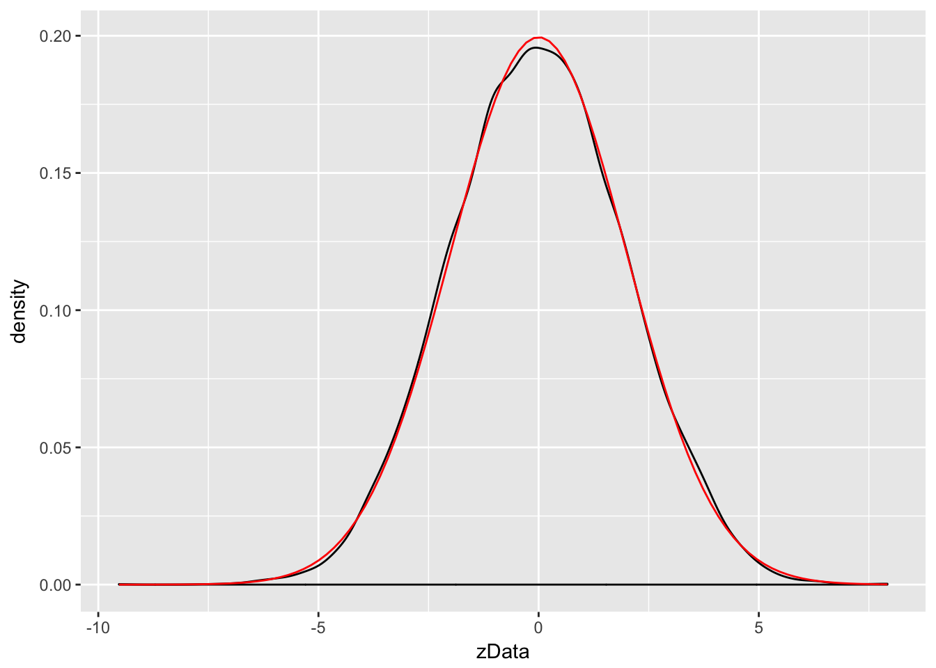
Wow! Those look really close to the same thing!
Example Let \(Z\) be a standard normal rv. Find the pdf of \(Z^2\) and compare it to the pdf of a \(\chi^2\) (chi-squared) rv with one degree of freedom. The distname for a \(\chi^2\) rv is chisq, and rchisq requires the degrees of freedom to be specified using the df parameter.
We plot the pdf of \(Z^2\) and the chi-squared rv with one degree of freedom on the same plot. \(\chi^2\) with one df has a vertical asymptote at \(x = 0\), so we need to explicitly set the \(y\)-axis scale:
zData <- rnorm(10000)^2
f <- function(x) dchisq(x, df=1)
ggplot(data.frame(zData), aes(x = zData)) +
  coord_cartesian(ylim = c(0,1.2)) +        # set y-axis scale
  geom_density() +
  stat_function(fun = f, color = "red")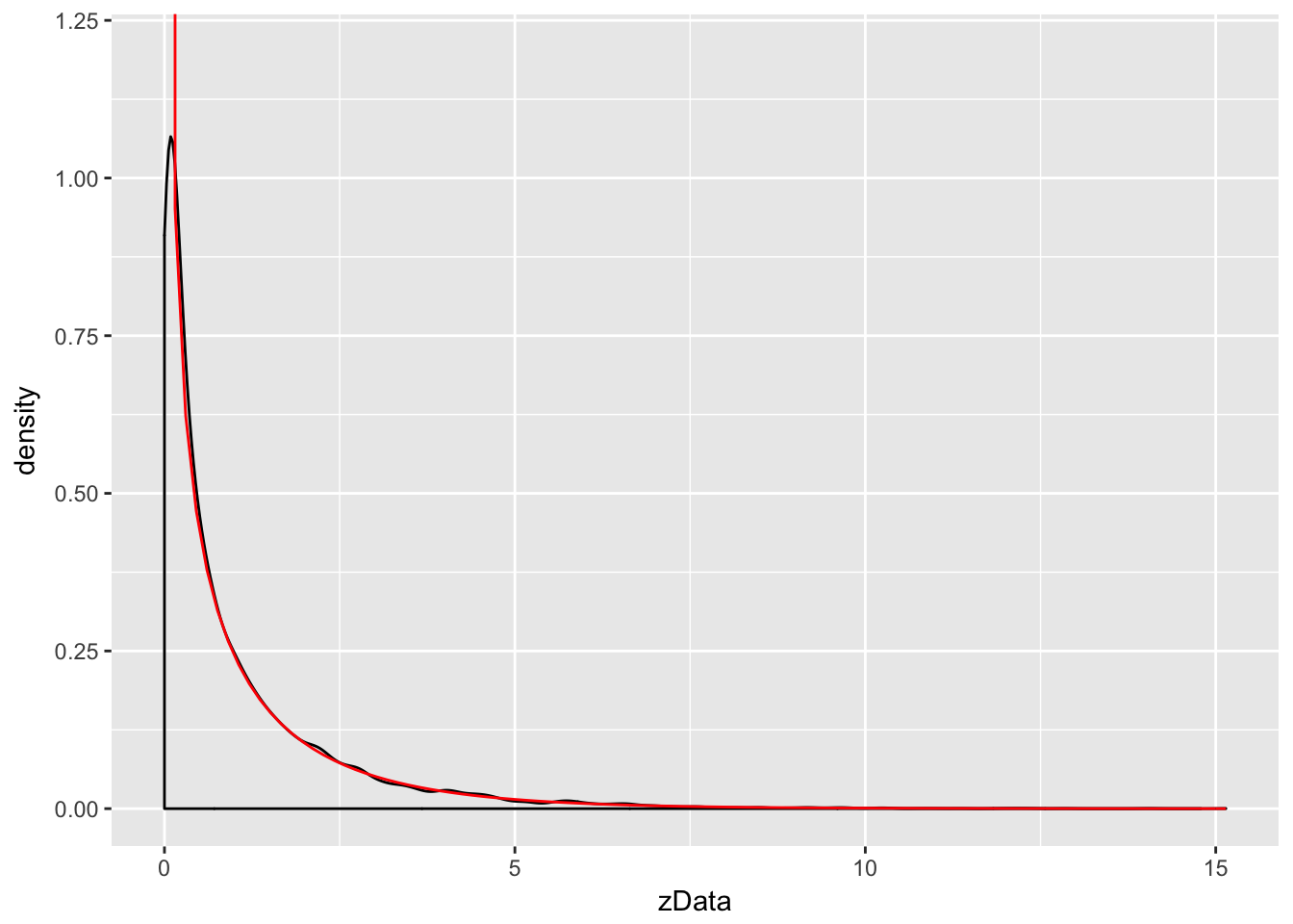
As you can see, the estimated density follows the true density quite well. This is evidence that \(Z^2\) is, in fact, chi-squared.
4.5 The Central Limit Theorem
We will not prove this theorem, but we will do simulations for several examples. They will all follow a similar format.
Example Let \(X_1,\ldots,X_{30}\) be Poisson random variables with rate 2. From our knowledge of the Poisson distribution, each \(X_i\) has mean \(\mu = 2\) and standard deviation \(\sigma = \sqrt{2}\). The central limit theorem then says that \[ \frac{\overline{X} - 2}{\sqrt{2}/\sqrt{30}} \] is approximately normal with mean 0 and standard deviation 1. Let us check this with a simulation.
This is a little but more complicated than our previous examples, but the idea is still the same. We create an experiment which computes \(\overline{X}\) and then transforms by subtracting 2 and dividing by \(\sqrt{2}/\sqrt{30}\).
Here is a single experiment:
xbar <- mean(rpois(30,2))
(xbar - 2)/(sqrt(2)/sqrt(30))
## [1] 0.6454972Now, we replicate and plot:
xbar <- replicate(10000, mean(rpois(30,2)))  # generate 10000 samples of xbar
poisData <- (xbar - 2)/(sqrt(2)/sqrt(30))
ggplot(data.frame(poisData), aes(x = poisData)) +
  geom_density() +
  stat_function(fun = dnorm, color = "red")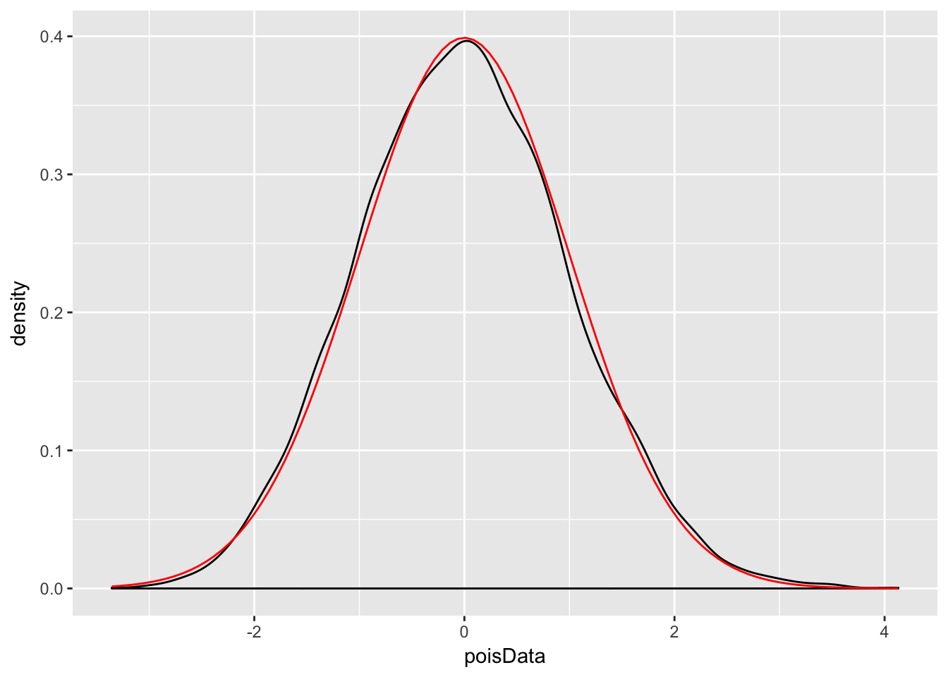
Very close!
Example Let \(X_1,\ldots,X_{50}\) be exponential random variables with rate 1/3. From our knowledge of the exponential distribution, each \(X_i\) has mean \(\mu = 3\) and standard deviation \(\sigma = 3\). The central limit theorem then says that \[ \frac{\overline{X} - 3}{3/\sqrt{50}} \] is approximately normal with mean 0 and standard deviation 1. We check this with a simulation.
xbar <- replicate(10000, mean(rexp(50,1/3)))   # generate 10000 samples of xbar
expData <- (xbar - 3)/(3/sqrt(50))
ggplot(data.frame(expData), aes(x = expData)) +
  geom_density() +
  stat_function(fun = dnorm, color = "red")
The Central Limit Theorem says that, if you take the mean of a large number of independent samples, then the distribution of that mean will be approximately normal. We call \(\overline{X}\) the sample mean because it is the mean of a random sample. In practice, if the population you are sampling from is symmetric with no outliers, then you can start to see a good approximation to normality after as few as 15-20 samples. If the population is moderately skew, such as exponential or \(\chi^2\), then it can take between 30-50 samples before getting a good approximation. Data with extreme skewness, such as some financial data where most entries are 0, a few are small, and even fewer are extremely large, may not be appropriate for the central limit theorem even with 500 samples (see example below). Finally, there are versions of the central limit theorem available when the \(X_i\) are not iid, but a single outlier of sufficient size invalidates the hypotheses of the Central Limit Theorem, and \(\overline{X}\) will not be normally distributed.
Example A distribution for which sample size of \(n = 500\) is not sufficient for good approximation via normal distributions.
We create a distribution that consists primarily of zeros, but has a few modest sized values and a few large values:
skewdata <- replicate(2000,0)                      # Start with lots of zeros
skewdata <- c(skewdata, rexp(200,1/10))            # Add a few moderately sized values
skewdata <- c(skewdata, seq(100000,500000,50000))  # Add a few large values

mu <- mean(skewdata)
sig <- sd(skewdata)
We use sample to take a random sample of size \(n\) from this distribution. We take the mean, subtract the true mean of the distribution, and divide by \(\sigma/\sqrt{n}\). We replicate that 10000 times. Here are the plots when \(\overline{X}\) is the mean of 100 samples:
n <- 100

xbar <- replicate(10000, mean( sample(skewdata, n, TRUE)) )
skewSample <- (xbar - mu)/(sig/sqrt(n))

ggplot(data.frame(skewSample), aes(x = skewSample)) +
  geom_density() +
  stat_function(fun = dnorm, color = "red")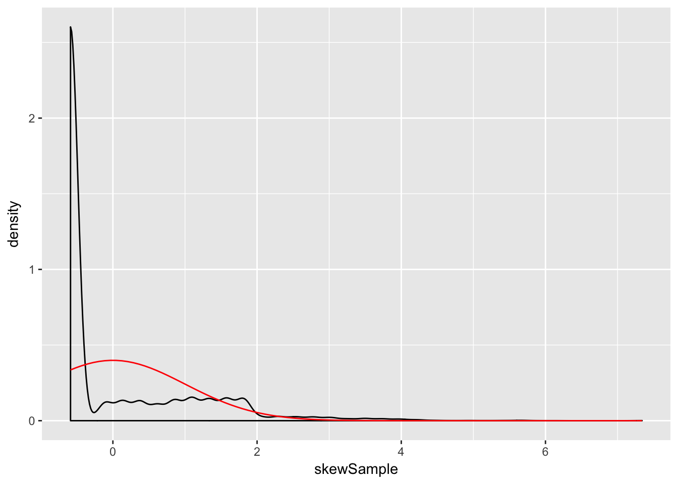
and 500 samples:
n <- 500

xbar <- replicate(10000, mean( sample(skewdata, n, TRUE)) )
skewSample <- (xbar - mu)/(sig/sqrt(n))

ggplot(data.frame(skewSample), aes(x = skewSample)) +
  geom_density() +
  stat_function(fun = dnorm, color = "red")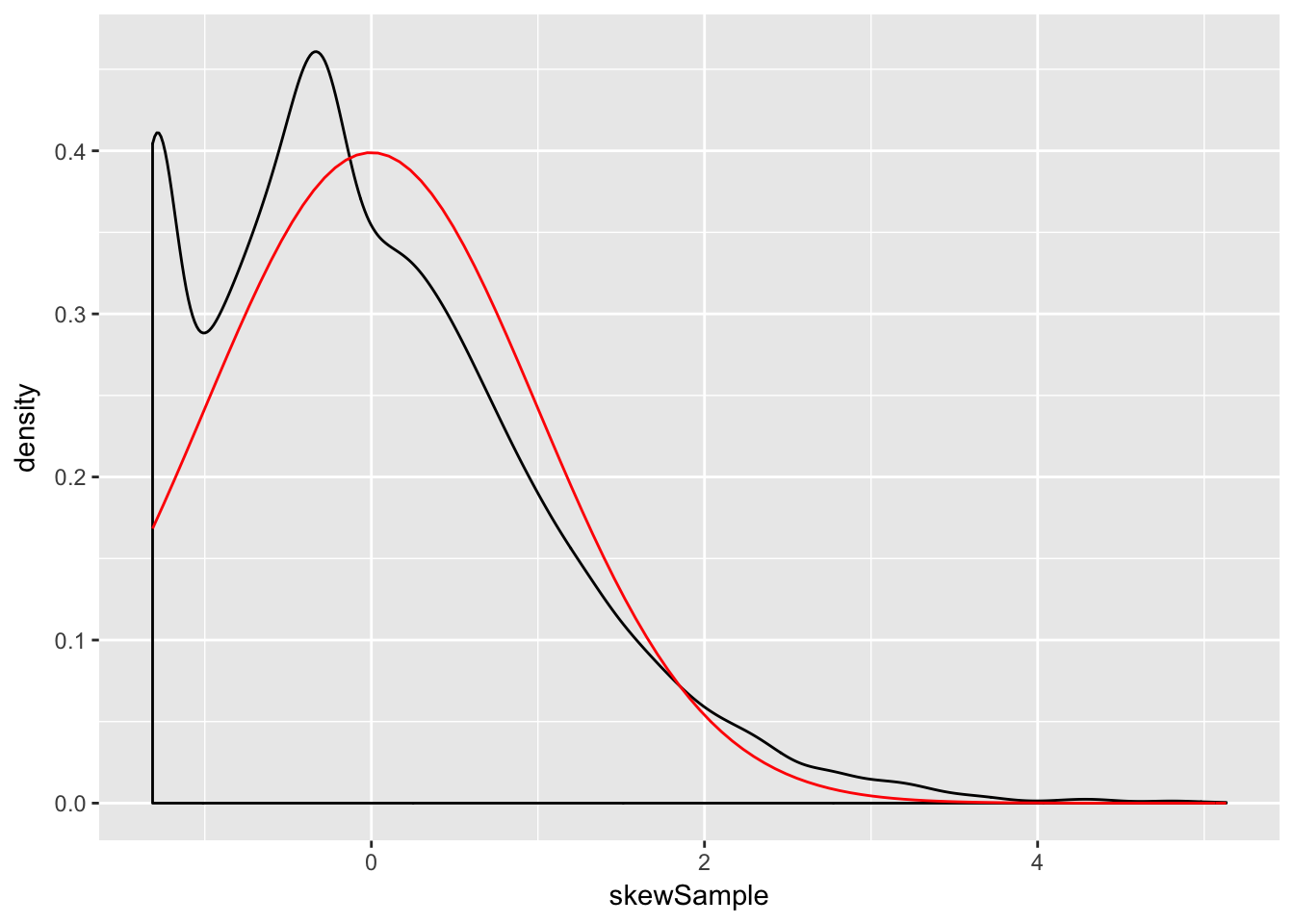
Even at 500 samples, the density is still far from the normal distribution, especially the lack of left tail. Of course, the Central Limit Theorem is still true, so \(\overline{X}\) must become normal if we choose \(n\) large enough:
n <- 5000

xbar <- replicate(10000, mean( sample(skewdata, n, TRUE)) )
skewSample <- (xbar - mu)/(sig/sqrt(n))

ggplot(data.frame(skewSample), aes(x = skewSample)) +
  geom_density() +
  stat_function(fun = dnorm, color = "red")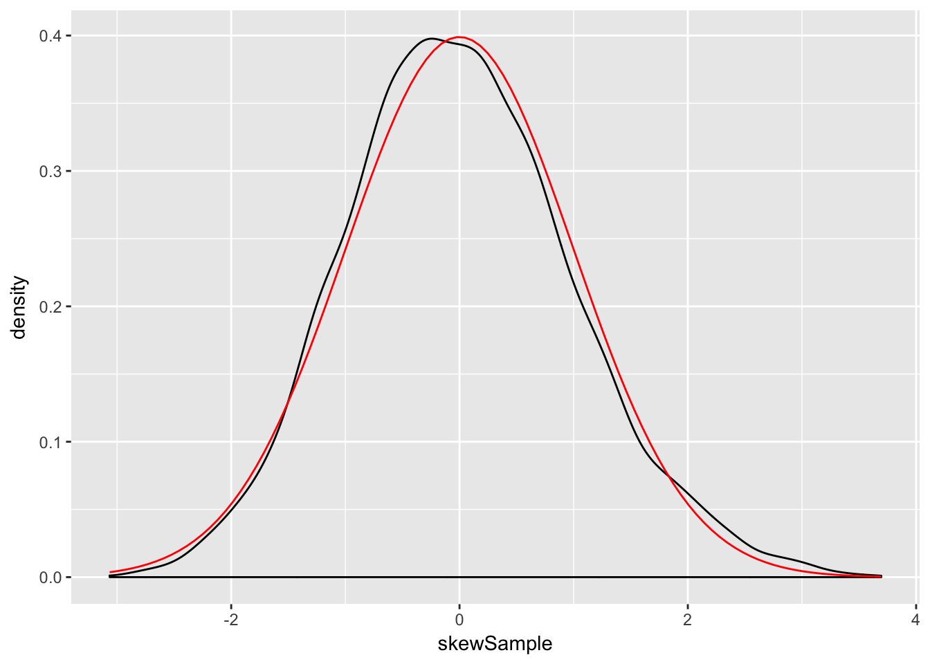
There may still be a slight skewness in this picture, but we are now very close to being normal.
4.6 Sampling Distributions (optional)
We describe \(t\), \(\chi^2\) and \(F\) in the context of samples from normal rv. Emphasis is on understanding relationship between the rv and how it comes about from \(\overline{X}\) and \(S\). The goal is for you not to be surprised when we say later that test statistics have certain distributions. You may not be able to prove it, but hopefully won’t be surprised either. We’ll use density estimation extensively to illustrate the relationships.
Given \(X_1,\ldots,X_n\), which we assume in this section are independent and identically distributed with mean \(\mu\) and standard deviation \(\sigma\), we define the sample mean \[ \overline{X} = \sum_{i=1}^n X_i \] and the sample standard deviation \[ S^2 = \frac 1{n-1} \sum_{i=1}^n (X_i - \overline{X})^2 \] We note that \(\overline{X}\) is an estimator for \(\mu\) and \(S\) is an estimator for \(\sigma\).
4.6.1 Linear combination of normal rv’s
Let \(X_1,\ldots,X_n\) be independent rvs with means \(\mu_1,\ldots,\mu_n\) and variances \(\sigma_i^2\). Then \[ E[\sum a_i X_i] = \sum a_i E[X_i] \] and \[ V(\sum a_i X_i) = \sum a_i^2 V(X_i) \] As a consequence, \(E[aX + b] = aE[X] + b\) and \(V(aX + b) = a^2V(X)\). An important special case is that if \(X_1,\ldots,X_n\) are iid with mean \(\mu\) and variance \(\sigma^2\), then \(\overline{X}\) has mean \(\mu\) and variance \(\sigma^2/n\).
In the special case that \(X_1,\ldots, X_n\) are normal random variables, much more can be said. The following theorem generalizes our previous result to sums of more than two random variables.
You will be asked to verify this via estimating densities in special cases in the exercises. The special case that is very interesting is the following:
4.6.2 Chi-squared
Let \(Z\) be a standard normal(0,1) random variable. An rv with the same distribution is \(Z^2\) is called a Chi-squared rv with one degree of freedom. The sum of \(n\) independent \(\chi^2\) rv’s with 1 degree of freedom is a chi-squared rv with \(n\) degrees of freedom. In particular, the sum of a \(\chi^2\) with \(\nu_1\) degrees of freedom and a \(\chi^2\) with \(\nu_2\) degrees of freedom is \(\chi^2\) with \(\nu_1 + \nu_2\) degrees of freedom.
We have already seen above that \(Z^2\) has an estimated pdf similar to that of a \(\chi^2\) rv. So, let’s show via estimating pdfs that the sum of a \(\chi^2\) with 2 df and a \(\chi^2\) with 3 df is a \(\chi^2\) with 5 df.
chi2Data <- replicate(10000, rchisq(1,2) + rchisq(1,3))
f <- function(x) dchisq(x, df = 5)
ggplot(data.frame(chi2Data), aes(x = chi2Data)) +
  geom_density() +
  stat_function(fun = f, color = "red")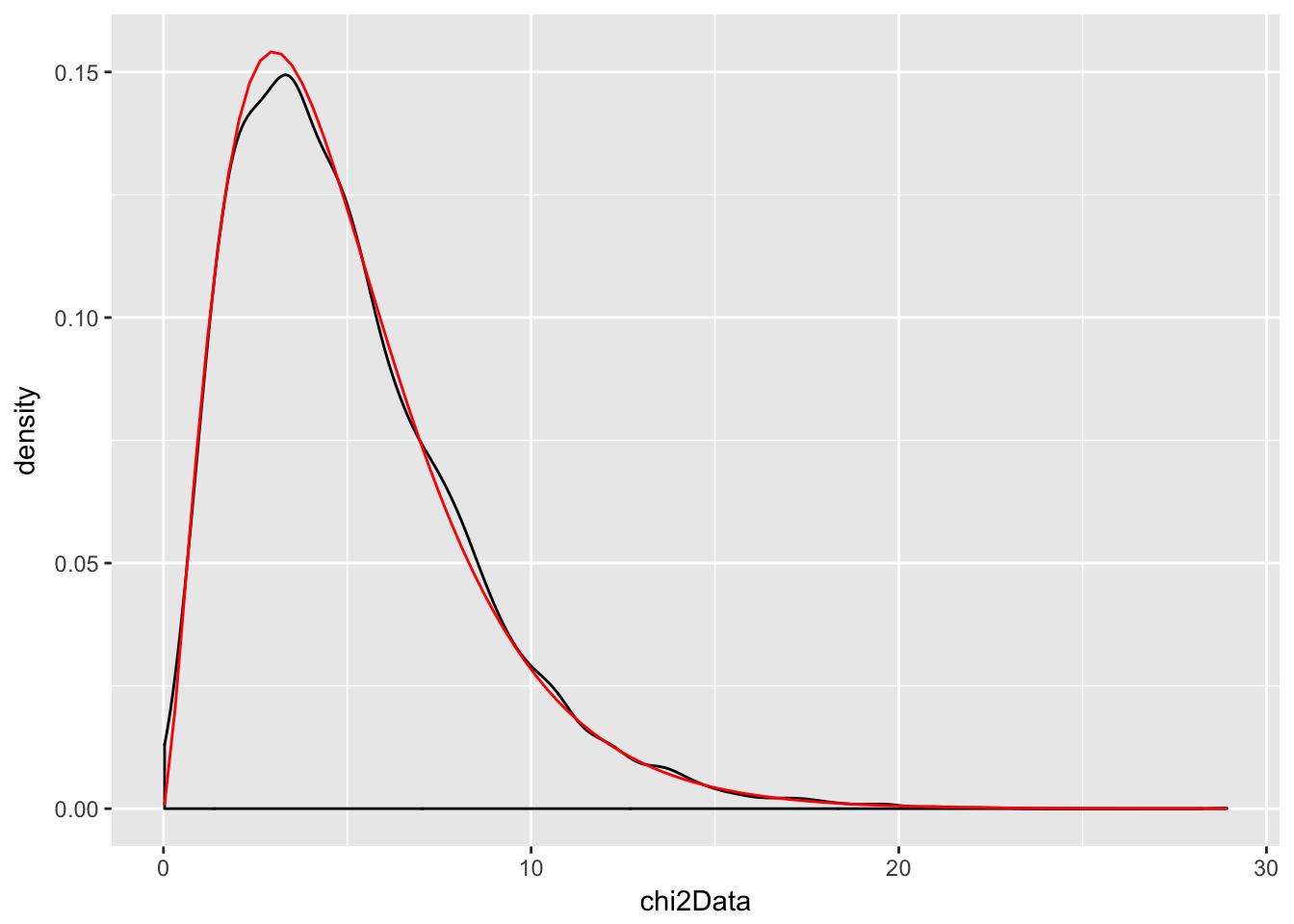
Example If \(X_1,\ldots,X_n\) are iid normal rvs with mean \(\mu\) and standard deviation \(\sigma\), then \[ \frac{n-1}{\sigma^2} S^2 \] is \(\chi^2_{n-1}\).
We provide a heuristic and a simulation as evidence. Heuristic: Note that \[ \frac{n-1}{\sigma^2} S^2 = \frac 1{\sigma^2}\sum_{i=1}^n (X_i - \overline{X})^2 \\ = \sum_{i=1}^n \bigl(\frac{X_i - \overline{X}}{\sigma}\bigr)^2 \] Now, if we had \(\mu\) in place of \(\overline{X}\) in the above equation, we would have exactly a \(\chi^2\) with \(n\) degrees of freedom. Replacing \(\mu\) by its estimate \(\overline{X}\) reduces the degrees of freedom by one, but it remains \(\chi^2\).
For the simulation of this, we estimate the density of \(\frac{n-1}{\sigma^2} S^2\) and compare it to that of a \(\chi^2\) with \(n-1\) degrees of freedom, in the case that \(n = 4\), \(\mu = 3\) and \(\sigma = 9\).
sdData <- replicate(10000, 3/81 * sd(rnorm(4, 3, 9))^2)
f <- function(x) dchisq(x, df = 3)
ggplot(data.frame(sdData), aes(x = sdData)) +
  geom_density() +
  stat_function(fun = f, color = "red")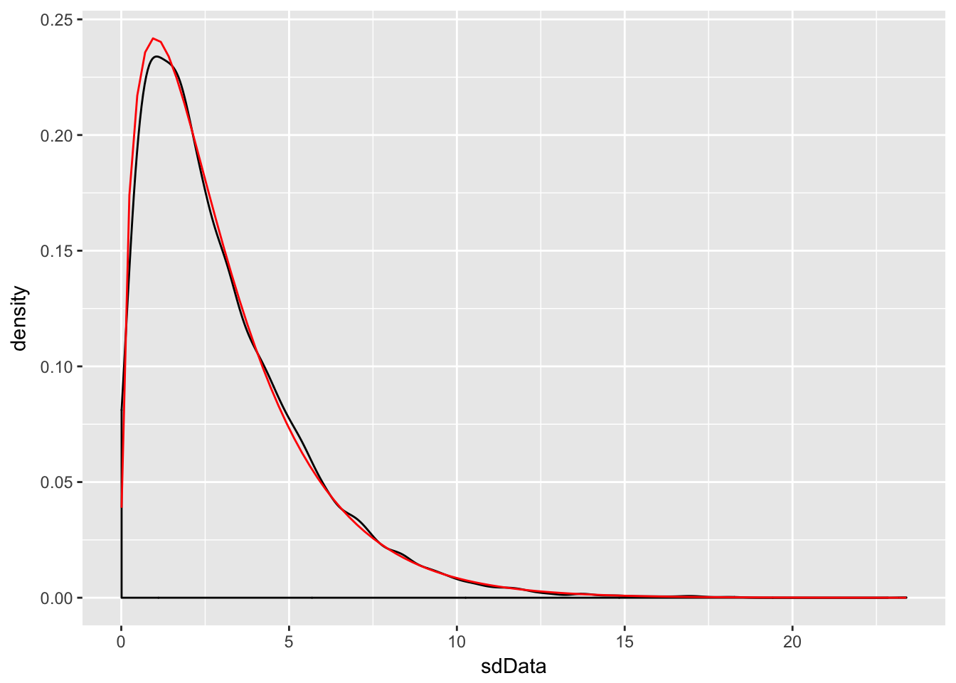
4.6.3 The \(t\) distribution
If \(Z\) is a standard normal(0,1) rv, \(\chi^2_\nu\) is a Chi-squared rv with \(\nu\) degrees of freedom, and \(Z\) and \(\chi^2_\nu\) are independent, then
\[ t_\nu = \frac{Z}{\sqrt{\chi^2_\nu/\nu}} \]
is distributed as a \(t\) random variable with \(\nu\) degrees of freedom.
Note that \(\frac{\overline{X} - \mu}{\sigma/\sqrt{n}}\) is normal(0,1). So, replacing \(\sigma\) with \(S\) changes the distribution from normal to \(t\).
Proof: \[ \frac{Z}{\sqrt{\chi^2_{n-1}/n}} = \frac{\overline{X} - \mu}{\sigma/\sqrt{n}}*\sqrt{\frac{\sigma^2 (n-1)}{S^2(n-1)}}\\ = \frac{\overline{X} - \mu}{S/\sqrt{n}} \] Where we have used that \((n - 1) S^2/\sigma^2\) is \(\chi^2\) with \(n - 1\) degrees of freedom.
Example Estimate the pdf of \(\frac{\overline{X} - \mu}{S/\sqrt{n}}\) in the case that \(X_1,\ldots,X_6\) are iid normal with mean 3 and standard deviation 4, and compare it to the pdf of the appropriate \(t\) random variable.
tData <- replicate(10000, {normData <- rnorm(6,3,4); (mean(normData) - 3)/(sd(normData)/sqrt(6))})
f <- function(x) dt(x, df = 5)
ggplot(data.frame(tData), aes(x = tData)) +
  geom_density() +
  stat_function(fun = f, color = "red")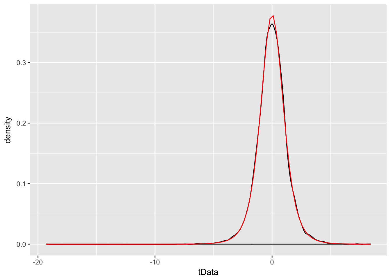
We see a very good correlation.
4.6.4 The F distribution
An \(F\) distribution has the same density function as \[ F_{\nu_1, \nu_2} = \frac{\chi^2_{\nu_1}/\nu_1}{\chi^2_{\nu_2}/\nu_2} \] We say \(F\) has \(\nu_1\) numerator degrees of freedom and \(\nu_2\) denominator degrees of freedom.
One example of this type is: \[ \frac{S_1^2/\sigma_1^2}{S_2^2/\sigma_2^2} \] where \(X_1,\ldots,X_{n_1}\) are iid normal with standard deviation \(\sigma_1\) and \(Y_1,\ldots,Y_{n_2}\) are iid normal with standard deviation \(\sigma_2.\)
4.6.5 Summary
- \(aX+ b\) is normal with mean \(a\mu + b\) and standard deviation \(a\sigma\) if \(X\) is normal with mean \(\mu\) and sd \(\sigma\).
- \(\frac{X - \mu}{\sigma}\sim Z\) if \(X\) is Normal(\(\mu, \sigma\)).
- \(\frac{\overline{X} - \mu}{\sigma/\sqrt{n}} \sim Z\) if \(X_1,\ldots,X_n\) iid normal(\(\mu, \sigma\))
- \(\lim_{n\to \infty} \frac{\overline{X} - \mu}{\sigma/\sqrt{n}} \sim Z\) if \(X_1,\ldots,X_n\) iid with finite variance.
- \(Z^2 \sim \chi^2_1\)
- \(\chi^2_\nu + \chi^2_\eta \sim \chi^2_{\nu + \eta}\)
- \(\frac{(n-1)S^2}{\sigma^2} \sim \chi^2_{n-1}\) when \(X_1,\ldots,X_n\) iid normal.
- \(\frac Z{\sqrt{\chi^2_\nu/\nu}} \sim t_\nu\)
- \(\frac{\overline{X} - \mu}{S/\sqrt{n}}\sim t_{n-1}\) when \(X_1,\ldots,X_n\) iid normal.
- \(\frac{\chi^2_\nu/\nu}{\chi^2_\mu/\mu} \sim F_{\nu, \mu}\)
- \(\frac{S_1^2/\sigma_1^2}{S_2^2/\sigma_2^2} \sim F_{n_1 - 1, n_2 - 1}\) if \(X_1,\ldots,X_{n_1}\) iid normal with sd \(\sigma_1\) and \(Y_1,\ldots,Y_{n_2}\) iid normal with sd \(\sigma_2\).
4.7 Point Estimators (Optional)
If \(X\) is a random variable that depends on parameter \(\beta\), then often we are interested in estimating the value of \(\beta\) from a random sample \(X_1,\ldots,X_n\) from \(X\). For example, if \(X\) is a normal rv with unknown mean \(\mu\), and we get data \(X_1,\ldots, X_n\), it would be very natural to estimate \(\mu\) by \(\frac 1n \sum_{i=1}^n X_i\). Notationally, we say \[ \hat \mu = \frac 1n \sum_{i=1}^n X_i = \overline{X} \] In other words, our estimate of \(\beta\) from the data \(x_1,\ldots, x_n\) is denoted by \(\hat \beta\).
The two point estimators that we are interested in at this point are point estimators for the \(mean\) of an rv and the \(variance\) of an rv. (Note that we have switched gears a little bit, because the mean and variance aren’t necessarily parameters of the rv. We are really estimating functions of the parameters at this point. The distinction will not be important for the purposes of this text.) Recall that the definition of the mean of a discrete rv with possible values \(x_i\) is \[ E[X] = \mu = \sum_{i=1}^n x_i p(x_i) \] If we are given data \(x_1,\ldots,x_n\), it is natural to assign \(p(x_i) = 1/n\) for each of those data points to create a new random variable \(X_0\), and we obtain \[ E[X_0] = \frac 1n \sum_{i=1}^n x_i = \overline{x} \] This is a natural choice for our point estimator for the mean of the rv \(X\), as well. \[ \hat \mu = \overline{x} = \frac 1n \sum_{i=1}^n x_i \]
Continuing in the same way, if we are given data \(x_1,\ldots,x_n\) and we wish to estimate the variance, then we could create a new random variable \(X_0\) whose possible outcomes are \(x_1,\ldots,x_n\) with probabilities \(1/n\), and compute \[ \sigma^2 = E[(X- \mu)^2] = \frac 1n \sum_{i=1}^n (x_i - \mu)^2 \] This works just fine as long as \(\mu\) is known. However, most of the time, we do not know \(\mu\) and we must replace the true value of \(\mu\) with our estimate from the data. There is a heuristic that each time you replace a parameter with an estimate of that parameter, you divide by one less. Following that heuristic, we obtain \[ \hat \sigma^2 = S^2 = \frac 1{n-1} \sum_{i=1}^n (x_i - \overline{x})^2 \]
4.7.1 Properites of Point Estimators
Note that the point estimators for \(\mu\) and \(\sigma^2\) can be thought of as random variables themselves, since they are combinations of a random sample from a distribution. As such, they also have distributions, means and variances. One property of point estimators that is often desirable is that it is unbiased. We say that a point estimator \(\hat \beta\) for \(\beta\) is unbiased if \(E[\hat \beta] = \beta\). (Recall: \(\hat \beta\) is a random variable, so we can take its expected value!) Intuitively, unbiased means that the estimator does not consistently underestimate or overestimate the parameter it is estimating. If were to estimate the parameter over and over again, the average value would converge to the correct value of the parameter.
Let’s consider \(\overline{x}\) and \(S^2\). Are they unbiased? It is possible to determine this analytically, and interested students should consult Wackerly et al for a proof. However, we will do this using R and simulation.
Example
Let \(X_1,\ldots, X_{5}\) be a random sample from a normal distribution with mean 1 and variance 1. Compute \(\overline{x}\) based on the random sample.
mean(rnorm(5,1,1))## [1] 1.674441You can see the estimate is pretty close to the correct value of 1, but not exactly 1. However, if we repeat this experiment 10,000 times and take the average value of \(\overline{x}\), that should be very close to 1.
mean(replicate(10000, mean(rnorm(5,1,1))))## [1] 1.000939It can be useful to repeat this a few times to see whether it seems to be consistently overestimating or underestimating the mean. In this case, it is not.
Variance
Let \(X_1,\ldots,X_5\) be a random sample from a normal rv with mean 1 and variance 4. Estimate the variance using \(S^2\).
sd(rnorm(5,1,2))^2## [1] 2.113989We see that our estimate is not ridiculous, but not the best either. Let’s repeat this 10,000 times and take the average. (We are estimating \(E[S^2]\).)
mean(replicate(10000, sd(rnorm(5,1,2))^2))## [1] 3.996854Again, repeating this a few times, it seems that we are neither overestimating nor underestimating the value of the variance.
For the sake of completeness, let’s show that \(\frac 1n \sum_{i=1}^n (x_i - \overline{x})^2\) is biased.
mean(replicate(10000, {data = rnorm(5,1,2); 1/5*sum((data - mean(data))^2)}))## [1] 3.212875If you run the above code several times, you will see that \(\frac 1n \sum_{i=1}^n (x_i - \overline{x})^2\) tends to significantly underestimate the value of \(\sigma^2 = 4\).
4.7.2 Variance of Unbiased Estimators
From the above, we can see that \(\overline{x}\) and \(S^2\) are unbiased estimators for \(\mu\) and \(\sigma^2\), respectively. There are other unbiased estimator for the mean and variance, however. For example, if \(X_1,\ldots,X_n\) is a random sample from a normal rv, then the median of the \(X_i\) is also an unbiased estimator for the mean. Moreover, the median seems like a perfectly reasonable thing to use to estimate \(\mu\), and in many cases is actually preferred to the mean. There is one way, however, in which the sample mean \(\overline{x}\) is definitely better than the median, and that is that it has a lower variance. So, in theory at least, \(\overline{x}\) should not deviate from the true mean as much as the median will deviate from the true mean, as measured by variance.
Let’s do a simulation to illustrate. Suppose you have a random sample of size 11 from a normal rv with mean 0 and standard deviation 1. We estimate the variance of \(\overline{x}\).
sd(replicate(10000, mean(rnorm(11,0,1))))^2## [1] 0.0913073Now we repeat for the median.
sd(replicate(10000, median(rnorm(11,0,1))))^2## [1] 0.1393718And, we see that the variance of the mean is lower than the variance of the median. This is a good reason to use the sample mean to estimate the mean of a normal rv rather than using the median, absent other considerations such as outliers.
4.8 Exercises
Five coins are tossed and the number of heads \(X\) is counted. Estimate via simulation the pmf of \(X\).
- Consider an experiment where 20 balls are placed randomly into 10 urns. Let \(X\) denote the number of urns that are empty.
- Estimate via simulation the pmf of \(X\).
- What is the most likely outcome?
- What is the least likely outcome that has positive probability?
Let \(X\) and \(Y\) be uniform random variables on the interval \([0,1]\). Estimate the pdf of \(X+Y\).
- Let \(X\) and \(Y\) be uniform random variables on the interval \([0,1]\). Let \(Z\) be the maximum of \(X\) and \(Y\).
- Estimate the pdf of \(Z\).
- From your answer to (a), decide whether \(P(0 \le Z \le 1/3)\) or \(P(1/3\le Z \le 2/3)\) is larger.
Let \(X_1,\ldots,X_{n}\) be uniform rv’s on the interval \((0,1)\). How large does \(n\) need to be before the pdf of \(\frac{\overline{X} - \mu}{\sigma/\sqrt{n}}\) is approximately that of a standard normal rv? (Note: there is no “right” answer, as it depends on what is meant by “approximately.” You should try various values of \(n\) until you find one where the estimate of the pdf is close to that of a standard normal.)
Let \(X_1,\ldots,X_{n}\) be chi-squared rv’s with 2 degrees of freedom. How large does \(n\) need to be before the pdf of \(\frac{\overline{X} - \mu}{\sigma/\sqrt{n}}\) is approximately that of a standard normal rv? (Hint: the wiki page on chi-squared will tell you the mean and sd of chi-sqaured rvs.)
The sum of two independent chi-squared rv’s with 1 degree of freedom is either exponential or chi-squared. Which one is it? What is the parameter associated with your answer?
The minimum of two exponential rv’s with mean 2 is an exponential rv. Use simulation to determine what the rate is.
Estimate the value of \(a\) such that \(P(a \le Y \le a + 1)\) is maximized when \(Y\) is the maximum value of two exponential random variables with mean 2.
(Requires optional section) Determine whether \(\frac 1n \sum_{i=1}^n (x_i - \mu)^2\) is a biased estimator for \(\sigma^2\) when \(n = 10\), \(x_1,\ldots,x_{10}\) is a random sample from a normal rv with mean 1 and variance 9.
(Requires optional section) Show through simulation that the median is an unbiased estimator for the mean of a normal rv with mean 1 and standard deviation 4. Assume a random sample of size 8.
Let \(X\) and \(Y\) be independent uniform rvs on the interval \([0,1]\). Estimate via simulation the pdf of the maximum of \(X\) and \(Y\), and compare it to the pdf of a beta distribution with parameters
shape1 = 2andshape2 = 1. (Usedbeta().)Estimate the density of the maximum of 7 uniform random variables on the interval \([0,1]\). This density is also beta; what are the parameters for the beta distribution?
- Consider the Log Normal distribution, whose root in R is
lnorm. The log normal distribution takes two parameters,meanlogandsdlog.- Graph the pdf of a Log Normal random variable with
meanlog = 0andsdlog = 1. The pdf of a Log Normal rv is given bydlnorm(x, meanlog, sdlog). - Let \(X\) be a log normal rv with meanlog = 0 and sdlog = 1. Estimate via simulation the density of \(\log(X)\), and compare it to a standard normal random variable.
- Estimate the mean and standard deviation of a Log Normal random variable with parameters 0 and 1/2.
- Using your answer from (b), find an integer \(n\) such that \[ \frac{\overline{X} - \mu}{\sigma/\sqrt{n}} \] is approximately normal with mean 0 and standard deviation 1.
- Graph the pdf of a Log Normal random variable with
Suppose 27 people write their names down on slips of paper and put them in a hat. Each person then draws one name from the hat. Estimate the expected value and standard deviation of the number of people who draw their own name. (Assume no two people have the same name!)
Is the product of two normal rvs normal? Estimate via simulation the pdf of the product of \(X\) and \(Y\), when \(X\) and \(Y\) are normal random variables with mean 0 and standard deviation 1. How can you determine whether \(XY\) is normal? Hint: you will need to estimate the mean and standard deviation.
(Hard) Suppose 6 people, numbered 1-6, are sitting at a round dinner table with a big plate of spaghetti, and a bag containing 5005 red marbles and 5000 blue marbles. Person 1 takes the spaghetti, serves themselves, and chooses a marble. If the marble is red, they pass the spaghetti to the left. If it is blue, they pass the spaghetti to the right. The guests continue doing this until the last person receives the plate of spaghetti. Let \(X\) denote the number of the person holding the spaghetti at the end of the experiment. Estimate the pmf of \(X\).
count(data.frame(x = replicate(10000, {birthdays <- sample(1:365, 50, replace = TRUE); sum(table(birthdays)[table(birthdays) > 1]) })), x) %>% mutate(prop = n/10000) %>% ggplot(aes(x, prop)) + geom_bar(stat = "identity")↩