8 Rank based tests

In Chapter 7 we saw how to create confidence intervals and perform hypothesis testing on population means. One of our takeaways, though, was that our techniques were inappropriate to use on populations with big outliers. In this section, we discuss rank based tests that can be used, and are still effective, when the population has these outliers.

8.1 One sample Wilcoxon Ranked-Sum Test

In this test, we will be testing $H_0: m = m_0$ versus $H_a: m\not= m_0$, where $m$ is the median of the underlying population. We will assume that the data is centered symmetrically around the median, so there can be outliers, bimodality or any kind of tails.

Let’s look at how the test works by hand by examining a simple, made up data set. Suppose you wish to test

\[ H_0: m = 6 \qquad {\rm vs} \qquad H_a: m\not=6 \] You collect the data $x_1 = 15, x_2 = 7, x_3 = 3, x_4 = 10$ and $x_5 = 13$. The test works as follows:

Compute $y_i = x_i - m_0$ for each $i$. We get $y_1 = 9, y_2 = 1, y_3 = -3, y_4 = 4$ and $y_5 = 7$.
Let $R_i$ be the rank of the absolute value of $y_i$. That is, $R_1 = 5, R_2 = 1, R_3 = 2, R_4 = 3, R_5 = 4$ since $R_1$ is largest, $R_2$ is smallest, etc.
Let $r_i$ be the signed rank of $R_i$; i.e. $r_i = R_i \times {\rm sign} (y_i)$. namely $r_1 = 5, r_2 = 1, r_3 = -2, r_4 = 3, r_5 = 4$
Add all of the positive ranks. We get $r_1 + r_2 + r_4 + r_5 = 13$. That is the test statistic for this test, and it is traditionally called $V$.
Compute the P-value for the test, which is the probability that we get a test statistic $V$ which is this, or more, unlikely under the assumption of $H_0$.

In order to perform the last step, we need to understand the sampling distribution of $V$, under the assumption of the null hypothesis, $H_0$. The ranks of our five data points will always be the numbers 1,2,3,4, and 5. When $H_0$ is true, each data point is equally likely to be positive or negative, and so will be included in the rank-sum half of the time. So, the expected value \[ E(V) = \frac{1}{2}\cdot 1 + \frac{1}{2}\cdot 2 + \frac{1}{2}\cdot 3 + \frac{1}{2}\cdot 4 + \frac{1}{2}\cdot5 = \frac{15}{2} = 7.5 \] In our example, $V = 13$, which is 5.5 away from the expected value of 7.5.

For the probability distribution of $V$, we list all $2^5 = 32$ possibilities of how the ranks could be signed. Since they are equally likely under $H_0$, we can compute the proportion that lead to a test statistic at least 5.5 away from the expected value of 7.5.

Table 8.1: All possible sums of positive signed ranks
r1	r2	r3	r4	r5	Sum of positive ranks	Far from 7.5?
-1	-2	-3	-4	-5	0	TRUE
-1	-2	-3	-4	5	5	FALSE
-1	-2	-3	4	-5	4	FALSE
-1	-2	-3	4	5	9	FALSE
-1	-2	3	-4	-5	3	FALSE
-1	-2	3	-4	5	8	FALSE
-1	-2	3	4	-5	7	FALSE
-1	-2	3	4	5	12	FALSE
-1	2	-3	-4	-5	2	TRUE
-1	2	-3	-4	5	7	FALSE
-1	2	-3	4	-5	6	FALSE
-1	2	-3	4	5	11	FALSE
-1	2	3	-4	-5	5	FALSE
-1	2	3	-4	5	10	FALSE
-1	2	3	4	-5	9	FALSE
-1	2	3	4	5	14	TRUE
1	-2	-3	-4	-5	1	TRUE
1	-2	-3	-4	5	6	FALSE
1	-2	-3	4	-5	5	FALSE
1	-2	-3	4	5	10	FALSE
1	-2	3	-4	-5	4	FALSE
1	-2	3	-4	5	9	FALSE
1	-2	3	4	-5	8	FALSE
1	-2	3	4	5	13	TRUE
1	2	-3	-4	-5	3	FALSE
1	2	-3	-4	5	8	FALSE
1	2	-3	4	-5	7	FALSE
1	2	-3	4	5	12	FALSE
1	2	3	-4	-5	6	FALSE
1	2	3	-4	5	11	FALSE
1	2	3	4	-5	10	FALSE
1	2	3	4	5	15	TRUE

The last column in Table 8.1 is TRUE if the sum of positive ranks is greater than or equal to 13 or less than or equal to 2. As you can see, we have 6 of the 32 possibilities are at least as far away from the test stat as our data, so the $p$-value would be $\frac{6}{32} = .1875$.

Let’s check it with the built in R command.

wilcox.test(c(15,7,3,10,13), mu = 6)

## 
##  Wilcoxon signed rank test
## 
## data:  c(15, 7, 3, 10, 13)
## V = 13, p-value = 0.1875
## alternative hypothesis: true location is not equal to 6

We see that our test statistic $V = 13$ and the $p$-value is 0.1875, just as we calculated.

In general, if you have $n$ data points, the expected value of $V$ is $E(V) = \frac{n(n+1)}{4}$ (Exercise 1) To deal with ties, give each data point the average rank of the tied values.

Let’s look at some examples. Consider the react data set. Recall that a t test looks like this:

react <- ISwR::react
t.test(react)

## 
##  One Sample t-test
## 
## data:  react
## t = -7.7512, df = 333, p-value = 1.115e-13
## alternative hypothesis: true mean is not equal to 0
## 95 percent confidence interval:
##  -0.9985214 -0.5942930
## sample estimates:
##  mean of x 
## -0.7964072

and we got a p-value of $10^{-13}$. If we instead were to do a wilcoxon test, we get

wilcox.test(react)

## 
##  Wilcoxon signed rank test with continuity correction
## 
## data:  react
## V = 9283.5, p-value = 2.075e-13
## alternative hypothesis: true location is not equal to 0

The p-value is the same order of magnitude, but is closer to double what the other p-value is. Each test is estimating the probability that we will obtain data this far away from $\mu = 0$, but they are summarizing what it means to be “this far away from $\mu = 0$” in different ways. If the underlying data really is normal, then the t test will be more likely to correctly determine that we can reject $H_0$ when we need to.

(p <- sum(replicate(10000,t.test(rnorm(50),mu=.5)$p.value)< .05))

## [1] 9375

Here, we see that t.test correctly rejects $H_0$ 93.75% of the time. Doing the same thing for Wilcoxon:

(p <- sum(replicate(10000,wilcox.test(rnorm(50),mu=.5)$p.value)< .05))

## [1] 9186

We see that Wilcoxon correctly rejects $H_0$ 91.86% of the time. So, if you have reason to think that your data is normal or symmetric with not too heavy tails, then you will get better results using t.test. If it is symmetric but with heavy tails or especially with outliers, then Wilcoxon will perform better.

8.2 Two Sample test

Next, we will be considering wilcox.test when we wish to compare the samples from two distributions (Mann-Whitney-Wilcoxon). We assume that all of the observations are independent for now; in particular, we are assuming we don’t have data that can naturally be matched in pairs (for now).

The null hypothesis is a little complicated to state:

$H_0$: the probability that an observation from sample 1 is larger than an observation from sample 2 is the same as the probability that an observation from sample 2 is larger than an observation from sample 1. That is, $P(X > Y) = P(Y > X)$. We may also rephrase this as a one-sided hypothesis by $P(X > Y) > P(Y > X)$, which would indicate that the values in the first sample are probably larger than the values in the second sample.

The alternative hypothesis is $H_a$ $P(X > Y) \not= P(Y > X)$ for the two-sided test, or $P(X > Y) \le P(Y > X)$ for the one-sided mentioned above.

The test statistic that we construct is the following: for each data point $x$ in Sample 1, we count the number of data points in Sample 2 that are less than $x$. The sum of “wins” is the test statistic. (Count ties as 0.5.) Under the null hypothesis, we expect the test statistic to come out to \[ N_1 N_2 /2. \] The function wilcox.test tells us whether the observed value of the test statistic is far enough away from the expected value to be statistically significant.

8.2.1 Example

In the data set mtcars, determine whether there is a difference in location of the displacement for automatic and manual transmission cars.

Let’s look at a boxplot:

ggplot(mtcars, aes(x = am, y = disp)) + geom_boxplot()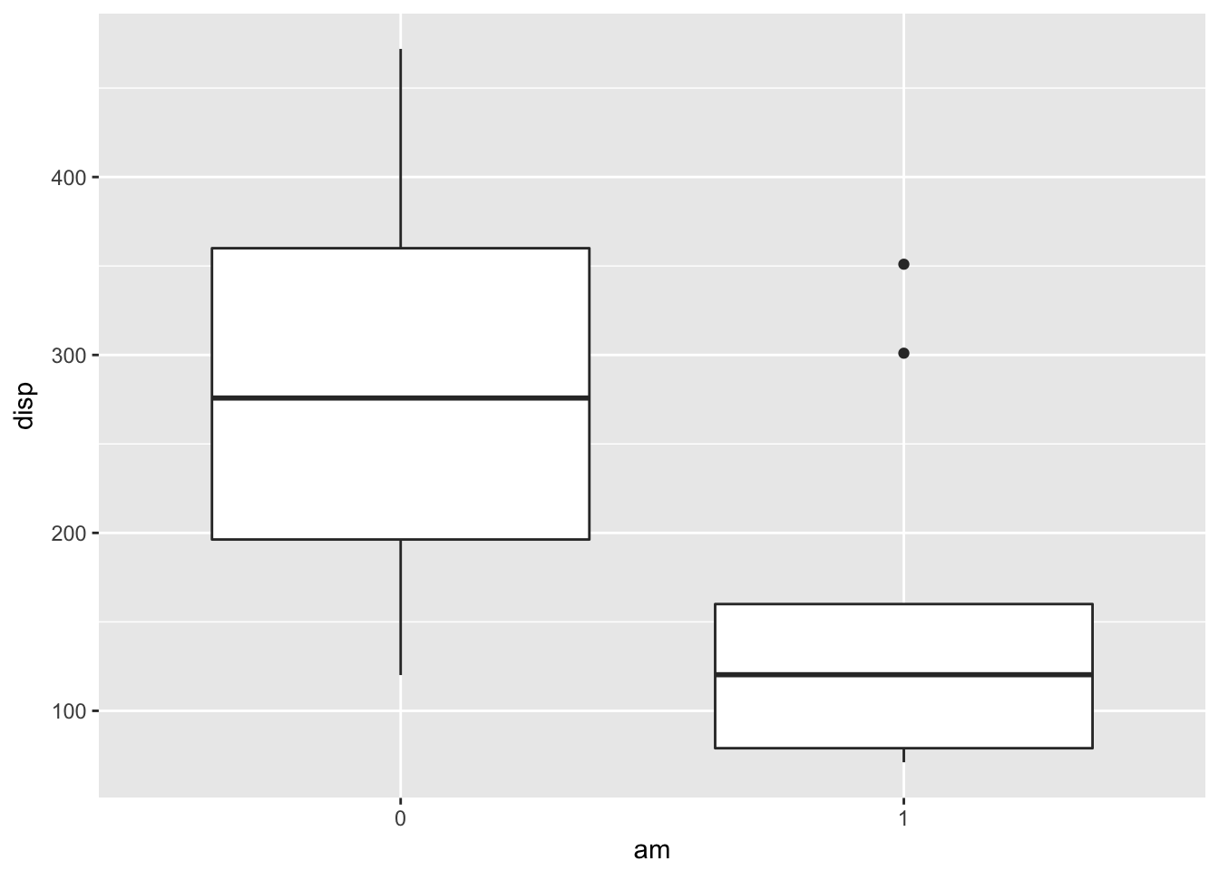

That’s no good. We forgot to tell R that am is actually a categorical variable.

mtcars$am <- as.factor(mtcars$am)
ggplot(mtcars, aes(x = am, y = disp)) + geom_boxplot()

There sure seems to be a difference in displacement based on that plot! It seems that automatics have higher displacement, but remember, we shouldn’t change our test to be one-sided based on the data that we observe. That would be cheating!

wilcox.test(disp~am, data = mtcars)

## Warning in wilcox.test.default(x = c(258, 360, 225, 360, 146.7, 140.8,
## 167.6, : cannot compute exact p-value with ties

## 
##  Wilcoxon rank sum test with continuity correction
## 
## data:  disp by am
## W = 214, p-value = 0.0005493
## alternative hypothesis: true location shift is not equal to 0

Note the use of ~ in wilcox.test; this is similar to its use in t.test, where we are telling R how we want to group the data contained in mtcars$disp.

If we store the result of the Wilcoxon test as

disp.wil <- wilcox.test(disp~am, data = mtcars)

## Warning in wilcox.test.default(x = c(258, 360, 225, 360, 146.7, 140.8,
## 167.6, : cannot compute exact p-value with ties

The test statistic can be pulled out with disp.wil$statistic = 214. This is much higher than the expected value of the test statistic under $H_0$, which was 123.5. (This means that displacement of auto beat displacement of manual more than expected under $H_0$). The $p$ value is disp.wil$p.value = 0.000549, which is quite low and we can reasonably reject $H_0$.

8.2.2 Ordinal Data

Another common use of wilcox.test is when the data is ordinal rather than numeric. Ordinal data is such that given data points $p_1$ and $p_2$, we can determine whether $p_1$ is bigger than $p_2$, less than $p_2$, or equal to $p_2$. However, we do not necessarily have a natural way of assigning numbers to the data points. Many people do assume there is a way of assigning numbers to the ordinal categories, but that doesn’t necessarily mean that it is a correct thing to do. For more information, see the somewhat whimsical book Do not use means with Likert scales.

A typical example of ordinal data is Likert-scale data. We have all seen surveys where we are asked to perform tasks such as:

Circle the response that most accurately reflects your opinion

Question	Strongly Agree	Agree	Netural	Disagree	Strongy Disagree
Pride and Prejudice is a great book	1	2	3	4	5
`wilcox.test` is a useful R command	1	2	3	4	5

Altough the options are listed as numbers, it does not necessarily make sense to treat the responses numerically. For example, if one respondant Strongly Disagrees that wilcox.test is useful, and another Strongly Agrees, is the mean of those responses Neutral? What is the mean of Strongly Agree and Agree? If the responses are numeric, what units do they have? So, it may not (and often does not) make sense to treat the responses to the survey as numeric data, even though it is encoded as numbers. However, we can order the responses in terms of amount of agreement as Strongly Agree > Agree > Disagree > Strongly Disagree. Note that I left out Neutral, because Neutral responses open a whole new can of worms. For example, we don’t know whether someone who put Neutral for Question (1) did so because the have never read Pride and Prejudice, or because they read it and don’t have an opinion on whether it is a great book. In once case, the response might better be treated as missing data, while in the other it would be natural to include the result between Agree and Disagree.

8.2.3 Example

Returning to the movieLens data, the number of stars that a movie receives as a rating can definitely be ordered from 5 stars being the most down to 1/2 star being the least. It is not as clear that the number of stars should be treated numerically, as it is more like asking whether a movie is Very Good, Good, OK, Bad or Very Bad. Consider the movies Toy Story and Toy Story II. Recall that the data that we have in our movie lens data set is a random sample from all users. Is there sufficient evidence to suggest that there is a difference in the ratings of Toy Story and Toy Story II in the full data set?

Before starting, we should decide whether we want to do a one-sided or a two-sided test. Some people have strong opinions about which Toy Story movie is better, but I don’t believe we have sufficient evidence or reason to do a one-sided test. So, let $X$ be the rating of Toy Story for a randomly sampled person in the large databaset. Let $Y$ be the rating of Toy Story II for a randomly sampled person. Our null and alternative hypotheses are

$H_0: P(X > Y) = P(Y > X) \\ H_a: P(X > Y) \not= P(Y > X)$

In order to do a two-sample Wilcoxon test, we need to load the data:

movies <- read.csv("http://stat.slu.edu/~speegle/_book_data/movieLensData", as.is = TRUE)

Now, we need to pull out the ratings that correspond to Toy Story and Toy Story II. We begin by finding the movieID of the Toy Story movies:

filter(movies, stringr::str_detect(Title, "Toy Story")) %>% select(MovieID, Title) %>% distinct()

##   MovieID              Title
## 1       1   Toy Story (1995)
## 2    3114 Toy Story 2 (1999)

Next, we create a data frame that only has the ratings of the Toy Story movies in it.

ts <- filter(movies, MovieID %in% c(1, 3114))

Now, we can perform the Wilcoxon test:

wilcox.test(Rating~Title, data = ts)

## 
##  Wilcoxon rank sum test with continuity correction
## 
## data:  Rating by Title
## W = 17188, p-value = 0.6162
## alternative hypothesis: true location shift is not equal to 0

And we can see that there is not a statistically significant difference in the ratings of Toy Story and Toy Story II, so we do not reject the null hypothesis.

8.2.4 Discussion

The primary benefit of using wilcox.test versus t.test is that the assumptions that we have made are weaker. For example, if your data is ordinal rather than numeric, it would not be appropriate to use a t-test without finding a statistically valid way of assigning the ordinal data to numerical values. However, the assumptions on wilcox.test are only that the data points can be compared to determine which is larger, so wilcox.test works just fine with ordinal data.

Wilcox.test in the two sample case is also more resistant to outliers than t.test, just as it is in the one-sample version. When your underlying data is normal, t.test will be more powerful. If your underlying data is not skewed, then typically at about 30 samples t.test works pretty well. When data is heavily skewed, you may need up to 100, 500 or even more samples before t.test is accurate. One down side of wilcox.test is that it is harder to interpret the alternative hypothesis; t.test has a nice, clean statement about the mean, while wilcox.test has a complicated looking statement about probabilities.

8.2.5 Example

This is an example of a paired, one-sided Mann-Whitney-Wilcoxon test. Let’s consider the anorexia data again, which is in the library MASS. We determine whether there is a difference in pre- and post- treatment weight of the subjects who underwent Cognitive Behavioral Treatment. Based on previous work, we expect that CBT will produce an increase in weight, so we use the one-sided test.

$H_0$ $P(X > Y) \ge P(Y > X)$ versus

$H_a$: $P(X > Y) < P(Y > X)$.

Let’s pull out the data that we want to examine:

cbt <- filter(MASS::anorexia, Treat == "CBT") 

#Used MASS:: so I didn't have to load entire library(MASS). You could also load the library if you prefer. But, MASS has a select function that will hide dplyr's select, if you load it afterwards.

We want to make a boxplot:

cbtBoxData <- gather(cbt, key = WeightTime, value = Weight, -Treat)
ggplot(cbtBoxData, aes(x = WeightTime, y = Weight)) + geom_boxplot()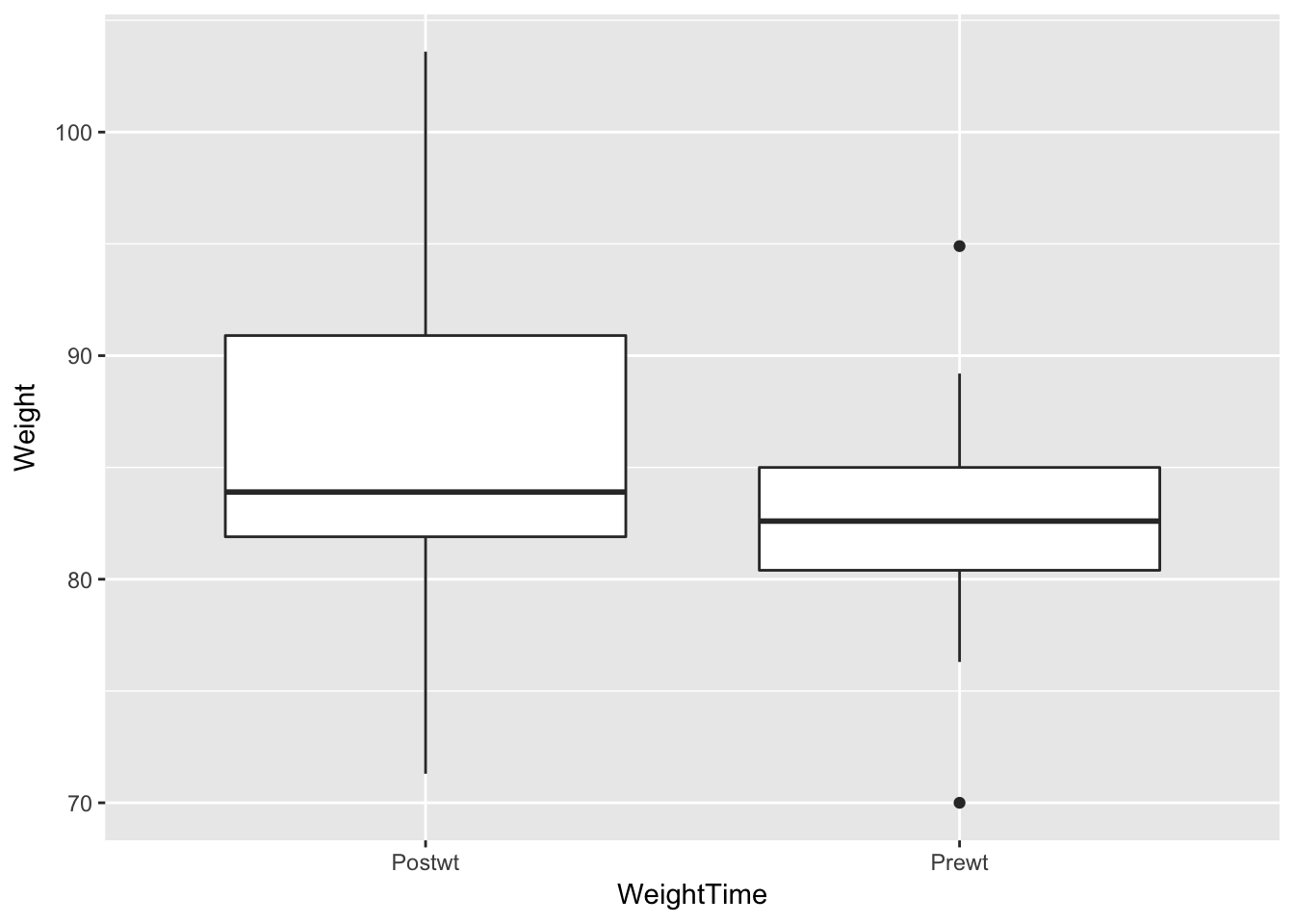

The boxplots are not conclusive. Perhaps there has been some increase, but it is not clear.

wilcox.test(cbt$Prewt, cbt$Postwt, paired = TRUE, alternative = "less")

## Warning in wilcox.test.default(cbt$Prewt, cbt$Postwt, paired = TRUE,
## alternative = "less"): cannot compute exact p-value with ties

## 
##  Wilcoxon signed rank test with continuity correction
## 
## data:  cbt$Prewt and cbt$Postwt
## V = 131.5, p-value = 0.03223
## alternative hypothesis: true location shift is less than 0

So, there is some evidence that the treatment was effective based on this test, but the evidence isn’t overwhelming. Note that if we hadn’t paired the data, we would have seen less significance in the results, and if we hadn’t done a one-sided test, then we would have seen even less significance.

wilcox.test(cbt$Prewt, cbt$Postwt, paired = FALSE, alternative = "less")

## Warning in wilcox.test.default(cbt$Prewt, cbt$Postwt, paired = FALSE,
## alternative = "less"): cannot compute exact p-value with ties

## 
##  Wilcoxon rank sum test with continuity correction
## 
## data:  cbt$Prewt and cbt$Postwt
## W = 320.5, p-value = 0.06088
## alternative hypothesis: true location shift is less than 0

wilcox.test(cbt$Prewt, cbt$Postwt, paired = FALSE, alternative = "two")

## Warning in wilcox.test.default(cbt$Prewt, cbt$Postwt, paired = FALSE,
## alternative = "two"): cannot compute exact p-value with ties

## 
##  Wilcoxon rank sum test with continuity correction
## 
## data:  cbt$Prewt and cbt$Postwt
## W = 320.5, p-value = 0.1218
## alternative hypothesis: true location shift is not equal to 0

These are examples of decisions that are made in analyzing data that can have large influences on the outcome of the analysis. It is important to think carefully about your data before going too far in your analysis. If you start playing around with different analyses, looking for one that shows something is significant, then you can end up with drastically underestimated probabilities of Type I errors. Think about it like this - most every data set has something about it that doesn’t happen too often. If you keep testing until you land on whatever that is, then you have only learned something about the underlying process if your result is reproducible. That’s not to say you can’t look for trends in data; you just need to be sure the trend you find is representative of all data of this type, and can be replicated in further experiments. The more different kinds of analyses you perform before finding something that is significant, the more questionable your result becomes.

8.3 Simulations

We begin by preparing the power of Wilcoxon rank-sum test with t-test when the underlying data is normal. We assume we are testing $H_0: \mu = 0$ versus $H_a: \mu \not= 0$ at the $\alpha = .05$ level, when the underlying population is truly normal with mean 1 and standard deviation 1 with a sample size of 10. Let’s first estimate the percentage of time that a t-test correctly rejects the null-hypothesis.

set.seed(1)
sum(replicate(10000, t.test(rnorm(10,1,1))$p.value < .05))

## [1] 7932

We see that we correctly reject $H_0$ 79.3% of the time in this simulation Let’s see what would have happened had we used Wilcoxon.

sum(replicate(10000, wilcox.test(rnorm(10,1,1))$p.value < .05))

## [1] 7845

Here, we see that we correctly reject $H_0$ 78.5% of the time in this simulation. If you repeat the simulations, you will see that indeed the t.test correctly rejects $H_0$ more often than the Wilcoxon test does, on average.

However, if there is a departure from normality in the underlying data, Wilcoxon can outperform t.test. Let’s repeat the above simulations in the case that we are sampling from a t distribution with 3 degrees of freedom that has been shifted to the right by one.

sum(replicate(10000, t.test(rt(10,3) + 1)$p.value < .05))

## [1] 5358

sum(replicate(10000, wilcox.test(rt(10,3) + 1)$p.value < .05))

## [1] 5423

Here, we see that Wilcoxon outperforms t, but not by a tremendous amount.

Note that we didn’t explain how to compute the $p$-value when using two-sample Wilcoxon. One way we can do it is via simulation. Let’s return to the mtcars example from above, and recall that we are testing the displacement versus the transmission. Let’s remind ourselves how many data points we have:

nrow(mtcars)

## [1] 32

sum(mtcars$am == "1")

## [1] 13

We have 13 with manual transmission and 19 with automatic transmission. If there were really no difference in the displacement for automatic and manual transmissions, then the ranks of the displacement would be assigned randomly. To simulate that, we imagine that we have 32 possible ranks, and we sample 13 of them to form the ranks of displacements for the manual transmissions.

manualRanks <- sample(32, 13)

The automatic ranks are the ones that are not in manualRanks. It can be a little tricky to pull these out. Here are a couple of ways:

which(!(1:32 %in% manualRanks))

##  [1]  2  3  5  6  8  9 10 11 12 13 17 18 19 20 21 23 25 29 32

 (1:32)[-manualRanks]

##  [1]  2  3  5  6  8  9 10 11 12 13 17 18 19 20 21 23 25 29 32

setdiff(1:32, manualRanks)

##  [1]  2  3  5  6  8  9 10 11 12 13 17 18 19 20 21 23 25 29 32

autoRanks <- setdiff(1:32, manualRanks)

Now, we need to compute the test statistic for this ranking. The easiest way is to use wilcox.test and pull it out from there.

wilcox.test(manualRanks, autoRanks)$statistic

##   W 
## 154

If it is bigger than or equal to the observed value of 214 or less than or equal to 33 (which is the value equally far from the expected value of 13*19/2 = 123.5), then the test statistic would be in the smallest rejection region that contains our observed test statistic. The $p$-value is the probability of landing in this rejection region, so we estimate it.

mean(replicate(20000, { manualRanks <- sample(32, 13);
                      autoRanks <- setdiff(1:32, manualRanks);
                      abs(wilcox.test(manualRanks, autoRanks)$statistic - 123.5) >= 90.5}))

## [1] 1e-04

Simulating these low probability events is not going to be extremely accurate. but we can say that the probability of getting a result that strong against the null hypothesis by change is very low. If you run the above code several times, you will see that it is between .0002 and .0005; so our estimate for the $p$-value based on this would be that it is somewhere in that range of values. Note that this is different than what wilcox.test returns, in part because we did not take into account ties in our simulation.

Another option would be to take the 32 data points that we have, and randomly assign them to either auto or manual transmissions, and estimate the $p$-value this way. The code would look like this: I am suppressing warnings in wilcox.test so we don’t get warned about ties so much!

mean(replicate(20000, {manualSample <- sample(32, 13) 
                      manualDisp <- mtcars$disp[manualSample];
                      autoDisp <- mtcars$disp[setdiff(1:32, manualSample)];
                      abs(suppressWarnings(wilcox.test(manualDisp, autoDisp)$statistic) - 123.5) >= 90.5}))

## [1] 3e-04

The results are similar to the previous method.

8.4 Exercises

Assume that $x_1,\ldots,x_n$ is a random sample from a symmetric distribution with mean 0.
1. Show that the expected value of the Wilcoxon test statistic $V$ is $\displaystyle E(V) = \frac{n(n+1)}{4}$
2. Find $\displaystyle \lim_{x_n\to \infty} E[V]$, which is the scenario of a single, arbitrarily large outlier.
This problem explores the effective type I error rate for a one sample Wilcoxon and t-tests. Choose a sample of 21 values where $X_1,\ldots,X_{20}$ are iid normal with mean 0 and sd 1, and $X_{21}$ is 10 or -10 with equal probability. Test $H_0: m = 0$ versus $H_a: m\not= 0$ at the $\alpha = .05$ level. How often does the Wilcoxon test reject $H_0$? Compare with the effective type I error rate for a t-test of the same data. Which test is performing closer to how it was designed?
This exercise explores how the Wilcoxon test changes when data values are transformed.
1. Suppose you wish to test $H_0: \mu = 0$ versus $H_0: \mu \not = 0$ using a Wilcoxon test You collect data $x_1 = -1,x_2 = 2,x_3 = -3,x_4 = -4$ and $x_5 = 5$. What is the $p$-value?
2. Now, suppose you multiply everything by 2: $H_0: \mu = 0$ versus $H_0: \mu\not = 0$ and your data is $x_1 = -2,x_2 = 4,x_3 = -6,x_4 = -8$ and $x_5 = 10$. What happens to the $p$-value? (Try to answer this without using R. Check your answer using R, if you must.)
3. Now, suppose you square the magnitudes of everything. $H_0: \mu = 0$ versus $H_a: \mu \not= 0$, and your data is $x_1 = -1,x_2 = 4,x_3 = -9,x_4 = -16$ and $x_5 = 25$. What happens to the $p$-value?
4. Compare your answers to the those that you got when you did the same exercise for $t$-tests in Exercise 7.8.
Consider the data in ex0221 in the Sleuth3 library. This data gives the Humerus length of 24 adult male sparrows that perished in a winter storm, as well as the Humerus length of 35 adult male sparrows that survived. The question under consideration is whether those that perished did so because of some physical characteristic; measured in this case by Humerus length.
1. Create a boxplot of Humerus length for the sparrows that survived and those that perished. Note that there is one rather extreme outlier in the Perished group.
2. Use a Wilcoxon ranked sum test to test whether the median Humerus length is the same in both groups.
3. Is there evidence to conclude that the Humerus length is different in the two groups?
Consider the data in ex0428 in the Sleuth3 library. This gives the plant heights in inches of plants of the same age, one of which was grown from a seed from a cross-fertilized flower, and the other of which was grown from a seed from a self-fertilized flower. Note that this data is in “wide” format rather than “long” format.
1. Use the command tidyr::gather(ex, key = Fertilization, value = height) to convert the data into long format.
2. Create a boxplot of the height of the flowers for each type of fertilization. Comment on any abnormalities apparent.
3. Is there a significant difference in the height of the flowers at the $\alpha = .05$ level?
Suppose you wish to test $H_0:\mu = 3$ versus $H_a: \mu\not= 3$. You collect the data points $x_1 = -1$, $x_2 = 0$, $x_3 = 2$ and $x_4 = 8$. Go through all of the steps of a Wilcoxon signed rank test and determine a $p$-value. Check your answer using R.
In this problem, we estimate the probability of a type II error. Suppose you wish to test $H_0:\mu = 1$ versus $H_a: \mu\not=1$ at the $\alpha = .05$ level.
1. Suppose the true underlying population is $t$ with 3 degrees of freedom, and you take a sample of size 20.
  1. What is the true mean of the underlying population?
  2. What type of error would be possible to make in this context, type I or type II? In the problems below, if the error is impossible to make in this context, the probability would be zero.
2. Approximate the probability of a type I error if you use a t test.
3. Approximate the probability of a type I error if you use a Wilcoxon test.
4. Approximate the probability of a type II error if you use a t test.
5. Approximate the probability of a type II error if you use a Wilcoxon test.
6. Note that t random variables with small degrees of freedom have heavy tails and contain data points that look like outliers. Does it appear that Wilcoxon or t is more powerful with this type of population?
How well can hypothesis tests detect a small change? Suppose the population is normal with mean $\mu = 0.1$ and standard deviation $\sigma = 1$. We test the hypothesis $H_0: \mu = 0$ versus $H_0: \mu \neq 0$.
1. When $n = 100$, what percent of the time does a t-test correctly reject $H_0$?
2. When $n = 100$, what percent of the time does a Wilcoxon test correctly reject $H_0$?
3. Repeat parts a and b with $n = 1000$.
4. The assumptions for both tests are satisfied, since the population is normal. Which test does a better job of rejecting the null hypothesis?