Chapter 7 Models

A model in dbt is any SQL file. It is what dbt will use to build tables, views and any other transformations in your data warehouse. In dbt, models are executed with the hit and run command: dbt run.

7.1 Running a model

dbt did us a very big favour during installation; it came with two models already created for us. These are namely the my_first_dbt_model.sql and my_second_dbt_model.sql within the models/example directory. It also provided a schema.yml file within the same directory which provides definitions for the models’ schema.

Alright. Assuming that you are within the dbt_book subdirectory and your virtual environment (venv) already activated, type dbt run in your terminal like so:

(venv) sammigachuhi@Gachuhi:~/dbt_book/dbt_book$ dbt run

This will initiate a series of printouts. However, before we go to the expected output, you may run into an error related to the location not being found.

404 Not found: Dataset dbt-project-437116:nyc_bikes was not found in location US; reason: notFound, message: Not found: Dataset dbt-project-437116:nyc_bikes was not found in location US

When we were initializing our project using dbt init we selected option 1 for US. Luckily, there is a work around to this. It involves editing the projects.yml file. If you run dbt debug it will also show the path of your projects.yml alongside other configuration information.

18:19:56  Running with dbt=1.8.7
18:19:56  dbt version: 1.8.7
18:19:56  python version: 3.10.12
18:19:56  python path: /home/sammigachuhi/dbt_book/venv/bin/python3
18:19:56  os info: Linux-5.15.153.1-microsoft-standard-WSL2-x86_64-with-glibc2.35
18:19:57  Using profiles dir at /home/sammigachuhi/.dbt
18:19:57  Using profiles.yml file at /home/sammigachuhi/.dbt/profiles.yml
--snip--

Go to the provided path for profiles.yml which, in my case, is found at the path - /home/sammigachuhi/.dbt. Open it and change the line with location to read from US to africa-south1.

dbt_book:
  outputs:
    dev:
      dataset: nyc_bikes
      job_execution_timeout_seconds: 300
      job_retries: 1
      keyfile: /home/sammigachuhi/dbt_credentials/dbt_book.json
      location: africa-south1 
--snip---

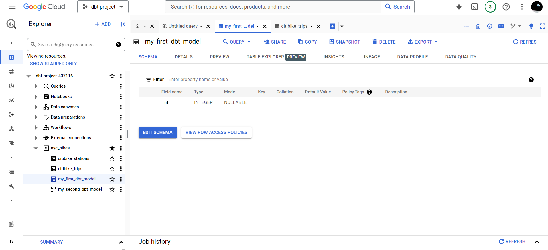
Now come back, and rerun dbt run again. dbt should now be able to run against your warehouse and create a table called my_first_dbt_model and a view my_second_dbt_model in BigQuery.

“How do I know that my queries ran successfully?”, you may ask. It is when the terminal prints out: Completed successfully. Beneath this message, will be a single line statement of the number of models ran and if there have been any errors. We had two models, so we expect to see this reflect in the log. And it did.

18:21:16  Running with dbt=1.8.7
18:21:17  Registered adapter: bigquery=1.8.2
18:21:17  Unable to do partial parsing because saved manifest not found. Starting full parse.
18:21:19  Found 2 models, 4 data tests, 479 macros
18:21:19  
18:21:22  Concurrency: 1 threads (target='dev')
18:21:22  
18:21:22  1 of 2 START sql table model nyc_bikes.my_first_dbt_model ...................... [RUN]
18:21:30  1 of 2 OK created sql table model nyc_bikes.my_first_dbt_model ................. [CREATE TABLE (2.0 rows, 0 processed) in 7.83s]
18:21:30  2 of 2 START sql view model nyc_bikes.my_second_dbt_model ...................... [RUN]
18:21:34  2 of 2 OK created sql view model nyc_bikes.my_second_dbt_model ................. [CREATE VIEW (0 processed) in 4.01s]
18:21:34  
18:21:34  Finished running 1 table model, 1 view model in 0 hours 0 minutes and 14.88 seconds (14.88s).
18:21:34  
18:21:34  Completed successfully
18:21:34  
18:21:34  Done. PASS=2 WARN=0 ERROR=0 SKIP=0 TOTAL=2

The second way, and the most obvious, is checking the results in your BigQuery data warehouse. If you see the table and view my_first_dbt_model and my_second_dbt_model respectively, the query ran successfully.

Models

It was that simple, isn’t it?

7.2 Model structure

Let’s take a look at the model my_first_dbt_model.sql.

{{ config(materialized='table') }}

with source_data as (

    select 1 as id
    union all
    select null as id

)

select *
from source_data

/*
    Uncomment the line below to remove records with null `id` values
*/

-- where id is not null

The line {{ config(materialized='table') }} tells dbt to make the output my_first_dbt_model as a table. Any configurations set at the model level will overide the overarching ones set at dbt_project.yml file.

If you quickly take a sneek peek at the dbt_project.yml file and scroll to the bottom, you will see this configuration:

models:
  dbt_book:
    # Config indicated by + and applies to all files under models/example/
    example:
      +materialized: view

This configuration simply says that for every model inside the dbt_book/example directory, materialize the result as a view¹. However, inside our my_first_dbt_model.sql file, we set the materialization as table. What is in the sql model will override what is in the dbt_project.yml. However, for my_second_dbt_model.sql, we didn’t specify the materialization. Therefore, by default, the materialization specified at the dbt_project.yml level will be used.

Materialization is the persistence of a model in the data warehouse.

The second part of our first model is the actual SQL statement.

with source_data as (

    select 1 as id
    union all
    select null as id

)

select *
from source_data

This is a WITH SQL statement. In very simple terms, the SQL statement in parentheses () is what is referenced as source_data. Once we define our SQL statement and close it with parentheses, we can now select the data referenced by source_data.

The SQL statements in parentheses is what is referred to as Common Table Expression (CTE). They were designed to simplify complex queries and be used in the context of a larger query.

The second model doesn’t have much to provide but it introduces a new trick: the ref function.

select *
from {{ ref('my_first_dbt_model') }}
where id = 1

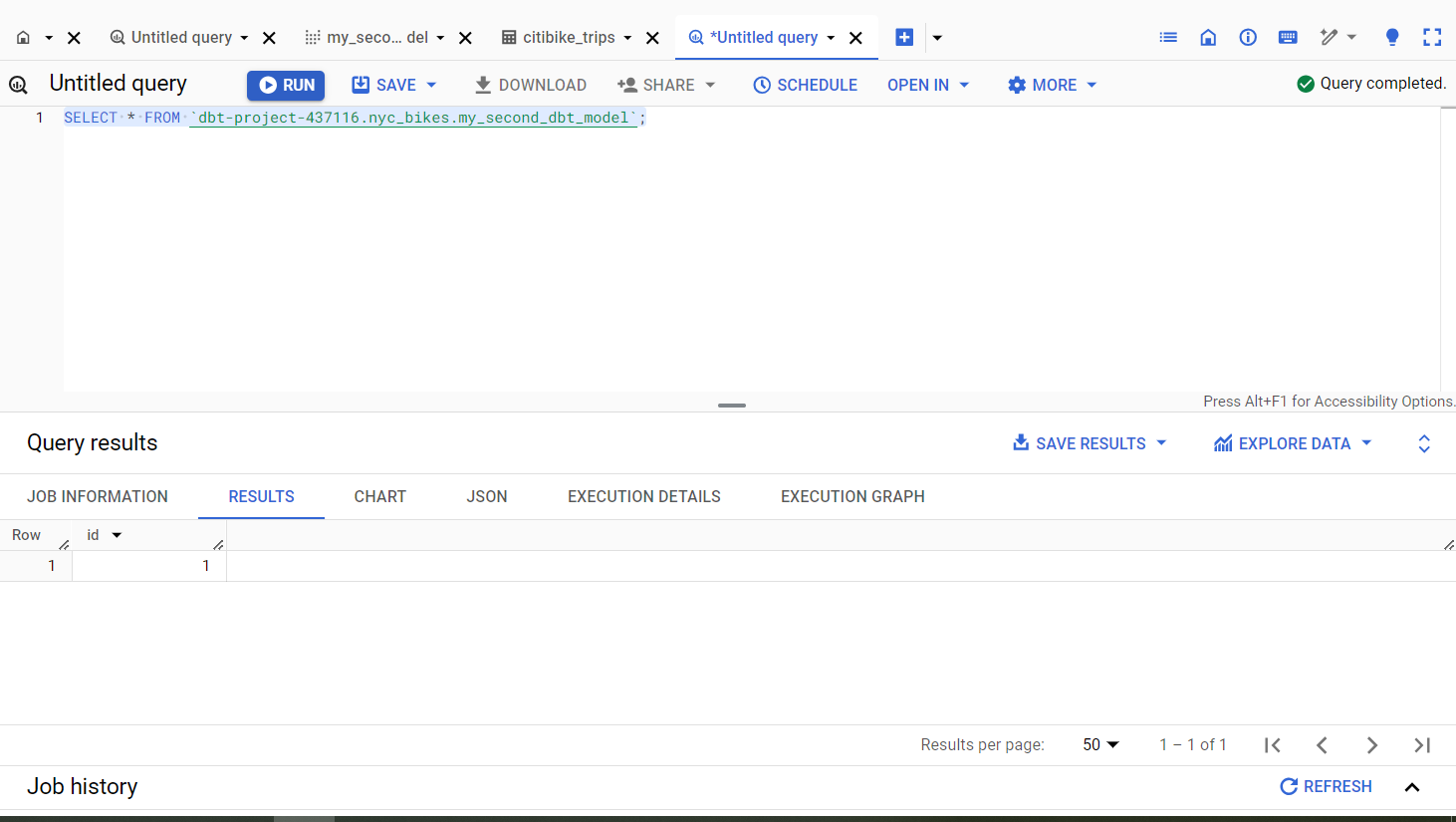
The ref function is part of the jinja templating language. It is used to reference a model that has been provided within the parentheses and enclosed with quotes (''). Therefore, in essence, our model simply returns the row(s) from my_first_dbt_model that contain the value 1 in the id column.

Here is the result of my_second_dbt_model view when I query BigQuery to show its contents.

Second model

7.3 A custom model

Now that we have seen how to run our models, it’s now time to fold our shirts and run our own custom model.

Let’s start easy. If you know SQL, there is no limit to the models, both in number and complexity, that you can do in dbt.

Our first model will endeavour to perform a change on the citi_trips table within our nyc_bikes dataset. In this dataset, there is a column called tripduration which shows the time in seconds for every cab trip. Humans prefer to read in minutes so a trivial dbt job would involve creating a column that shows the tripduration in minutes. By doing so, dbt would be performing the Transform part in the ELT.

In the citi_trips_minutes.sql model, we have written a code that creates a view of this result. Remember, views are just virtual tables but they do save on storage!

{{ config(materialized='view') }}

WITH citi_trips AS (
    SELECT *, 
    tripduration / 60 AS trip_duration_min
    FROM 
    `dbt-project-437116.nyc_bikes.citibike_trips` 
)

SELECT * FROM citi_trips

The above SQL statement is also a form of Common Table Expression (CTE). The variable citi_trips just references the SQL statement in parentheses.

There is another small trick of the trade. What if this very simple dbt model was just part of thousands, and longer running SQL models? Would we have to run the entire lot of models? No. To run only a specific model we use the --select keyword.

Below we run the citi_trips_minutes model.

dbt run --select models/example/citi_trips_minutes.sql

Below is the output.

Concurrency: 1 threads (target='dev')
18:50:33  
18:50:33  1 of 1 START sql view model nyc_bikes.citi_trips_minutes ....................... [RUN]
18:50:37  1 of 1 OK created sql view model nyc_bikes.citi_trips_minutes .................. [CREATE VIEW (0 processed) in 4.53s]
18:50:37  
18:50:37  Finished running 1 view model in 0 hours 0 minutes and 8.17 seconds (8.17s).
18:50:37  
18:50:37  Completed successfully
18:50:37  
18:50:37  Done. PASS=1 WARN=0 ERROR=0 SKIP=0 TOTAL=1

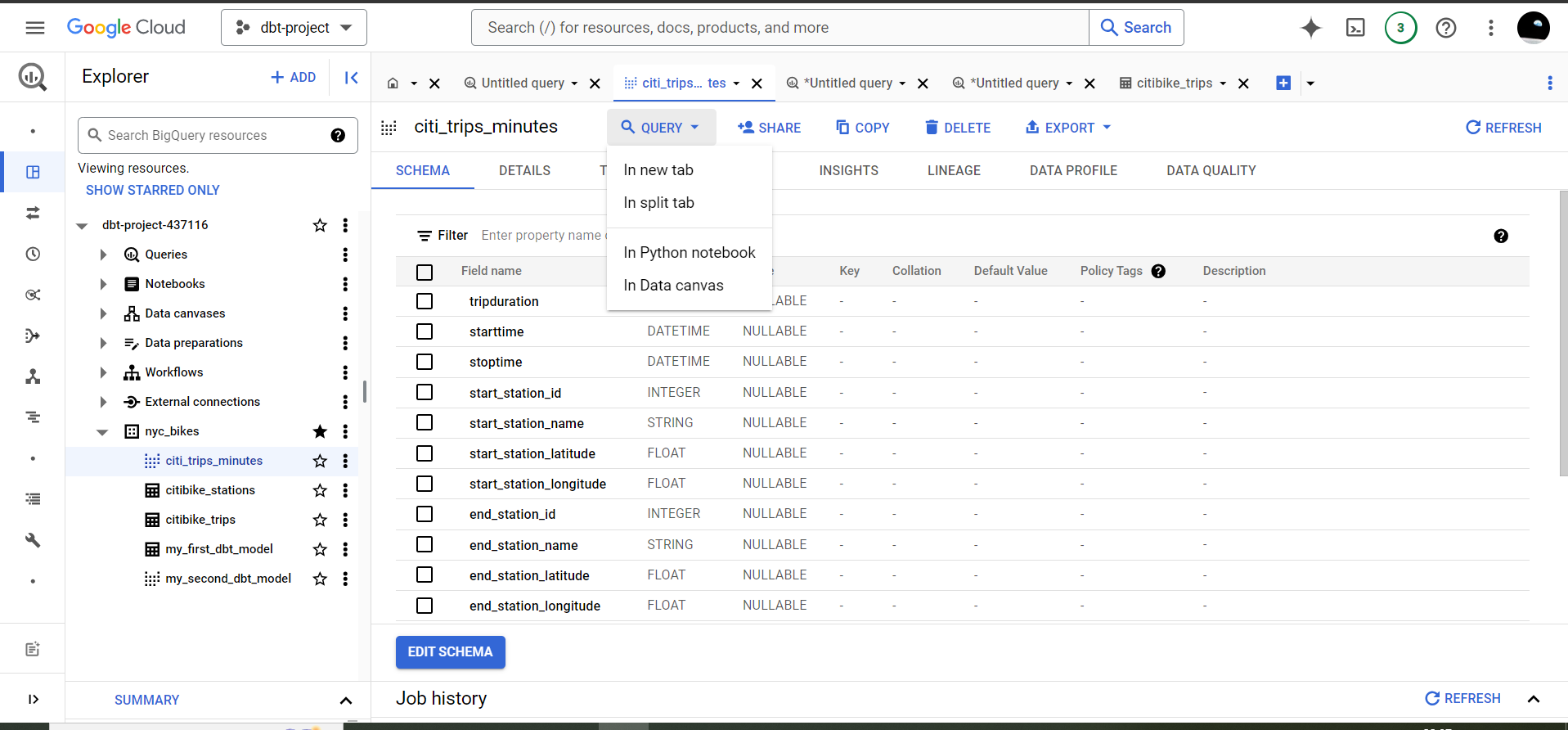
We are always glad when we see the soothing words “Completed successfully”. If you go to BigQuery, you will see a new view citi_trips_minutes already created. By default, the name of the newly formed view or table in the data warehouse will be that of the model used to create it.

Similar to the above, the below run command will also work. It doesn’t have the file type (.sql) suffix.

dbt run --select citi_trips_minutes

But how do we view this newly created result. Unlike a table, BigQuery does not offer the PREVIEW button. However, there is a way…

Query

Click on the Query button, select In new tab and a new tab will form. Copy this SQL query onto the tab and run it to display the result of our citi_trips_minutes view.

SELECT * FROM `dbt-project-437116.nyc_bikes.citi_trips_minutes` 

Our trip_duration_min column of interest is onto the far right of our view.

We had hinted earlier that there is no limit to the complexity or number of models you can create in dbt. Below is a more complex model. This model not only rounds off the minutes to one decimal place but also removes the null columns, thus reducing number of rows from 58,937,715 to 53,108,721. The model is saved as citi_trips_round.sql.

{{ config(materialized='view') }}

WITH citi_trips_round AS (
    SELECT *, ROUND(trip_duration_min, 1) AS trip_min_round
    FROM (
        SELECT *, 
        tripduration / 60 AS trip_duration_min
        FROM 
        `dbt-project-437116.nyc_bikes.citibike_trips`
        ) 
    WHERE tripduration IS NOT NULL
)

SELECT * FROM citi_trips_round

Our model is saved as the citi_trips_round view in BigQuery.

Create a new query tab in BigQuery to view the results. Also use the query tab to count the number of rows and compare them to those from the citibike_trips table. About 5.8 million rows with null value have been removed.

SELECT * FROM `dbt-project-437116.nyc_bikes.citi_trips_round`; 

SELECT COUNT(*) FROM `dbt-project-437116.nyc_bikes.citi_trips_round`;

-- This is the count of the original citibike_trips table
SELECT COUNT(*) FROM `dbt-project-437116.nyc_bikes.citibike_trips`;

You may be wondering what’s the advantage that dbt provides. After all, can’t one just use the SQL Query tab in BigQuery just to do the transformations and save the table? Fine, that can work. However, dbt offers a form of persistence to your models. Though modifiable like those in BigQuery, they can be versioned when saved into a code versioning platform like Github.

One more thing, you don’t have to use the models/example folder. You can choose to rename this one, or save the two models we created in a different folder. They will still run fine.

Create a new folder within the models directory called my_models. Move the citi_trips_minutes and citi_trips_round models into the my_models directory. Thereafter, run these two models using dbt run --select models/my_models. The models should run just fine.

As an extra bit of information, all successfully compiled and ran models will appear under the /target directory.

---

1. A view is a virtual table, similar to the original table, the physical dataset it was created from↩︎