8 Theory, prediction and application

Maria Paniw , Roger Cousens , Chris Baker and Thao Le

How to cite this chapter

Paniw M., Cousens R. D., Baker C. M. and Le T. P. (2023) Theory, prediction and application. In: Cousens R. D. (ed.) Effective ecology: seeking success in a hard science. CRC Press, Taylor & Francis, Milton Park, United Kingdom, pp. 127-150. Doi:10.1201/9781003314332-8

Abstract Prediction plays a central role in ecological research and application. Predictions can be used to test our models against emerging empirical data and to provide a scientific basis to guide future management decisions. However, there are many challenges to overcome to make accurate and useful predictions. How do we test the predictions of theoretical population models? What decisions do we need to make when attempting to predict abundance from empirical data? How can we make our predictions useful for our stakeholders? Predictions require ecological models, along with specialist skills, and data, which are often sparse. Complexity is not a guarantee of accuracy, and different management decisions will suffice with different levels of precision. In this chapter we examine such issues that ecologists face when trying to predict the dynamics of populations. We provide five case studies on predator-prey cycles, population spread modelling, animal abundance modelling, modelling for policy using decision science and adaptive management of threatened species.

8.1 A place for modelling in ecology

Prediction has a prominent place in both fundamental and applied ecology. In principle, we learn from using our knowledge to make predictions and then comparing those predictions with what we observe. If our predictions are good, then we can be reassured that our knowledge may be reasonable; if predictions are poor, then we may need to reconsider what we think we know. Peters (1991) was of the view that the ability to make predictions is the yardstick by which all scientific theories should be measured, while Houlahan et al. (2017) considered prediction to be the only way to demonstrate scientific understanding.

The need for predictions is also becoming increasingly more important. Anthropogenic environmental change is fundamentally altering natural systems, and we have a responsibility to alleviate the impacts that we cause. Ecological forecasting (near-term predictions that can be validated with independent data) has therefore emerged as a research frontier, with a primary focus on robustly and iteratively testing ecological predictions across different ecological scales (Dietze et al. 2018). If we can demonstrate that our predictions are trustworthy – according to some appropriate assessment – then we should be able to tell managers what the implications of their decisions are likely to be, i.e. what is likely to happen if they conduct some form of intervention.

Ecological prediction is inextricably linked to models. Models are inevitably simplifications of the real world that we hope capture the essence of nature, using the abstract tools of mathematics. They are a way of formulating a best guess based on our current ideas and information. But there are always potential errors involved in prediction: our data are limited and subject to uncertainty, we are forced to make assumptions and simplifications, and our ecological understanding will always be imperfect.

Realistically, there will always be limits to how accurate and precise our models and predictions can be. However, the process of modelling is, itself, an educational exercise and we learn a great deal simply from putting the model together, encapsulating our knowledge in a few succinct terms and subsequently seeing what is predicted. We also learn a great deal from our failures to predict, perhaps even more than when our predictions turn out to be good. Scientists in general learn a great deal from their mistakes (Bronowski 1979) – a fact of life that the public may not be keen to hear!

There are many different types of models – we will deal with some aspects of their structure in the next section. There are also many different uses of models. One important distinction is between predictions sensu stricto and projections: these are commonly confused but are quite different. Predictions are a model’s ability to reflect the observed data while assuming that those conditions will persist. Projections, on the other hand, refer to a model’s ability to reflect future dynamics of the system under plausible sets of conditions, i.e. under various scenarios proposed by the modeller or their stakeholders that deviate from previously observed conditions. Projections typically cannot be validated with independent data in the near-term.

An obvious example is the distinction between weather forecasts and climate-change projections. The former predict, over a short time window, what will happen if current trends persist, whereas the latter project what would happen under certain scenarios of greenhouse-gas emission such as those considered by the Intergovernmental Panel on Climate Change. More complex models that account for mechanisms may be relatively worse at replicating past observed trends but better at forecasting or projecting when compared with those models that merely assess patterns within data (Hefley et al. 2017).

Merely using a model to make a prediction or a projection is rarely a sufficient outcome, unless the aim is to demonstrate a new technique. The modeller needs to produce predictions that are reliable enough for the task at hand. We often have ethical responsibilities for our work: if we make a prediction that turns out to be inaccurate, we might cause an ecosystem to collapse, a species to go extinct or an enterprise to lose money. Users of the predictions also need to develop a rigorous opinion of what models tell them: just because a model gives a certain answer (perhaps the one that they were expecting) does not necessarily mean that it will be reliable, no matter how sophisticated or biologically realistic the model. It is easy to become over-confident.

So, how good does a decision-maker need a prediction to be for it to be useful to them? Or alternatively, how wrong are they prepared to be? This important design criterion seldom seems to be considered explicitly in ecological research. From a pragmatic perspective, models might not need to be highly accurate: an improvement of the quality of prediction in comparison with the status quo might be regarded as a worthwhile investment.

But, if we are to satisfy both ourselves and our peers, we still need to be able to assess the quality of a prediction, to measure any improvement that we have achieved and to base model selection on objective criteria. Obviously, the better the prediction is, or the more often it is accurate enough, then the more confident we will be in any recommendations that we make.

It is a worthwhile exercise for a modeller to consider how good they can expect their predictions to be and where improvements will come from: otherwise, they may be chasing a quality of prediction that is almost impossible to achieve. Improvements to prediction might come from several avenues, for example: future technical advances in programming and mathematics; the collection of more data (and with reduced bias that can improve our estimation of parameter values); changes to the model’s structure (either greater elaboration in order to make it more realistic or simplification to make it more tractable); or from replacing proxy variables by directly relevant variables (Yates et al. 2018). However, there will always be trade-offs to be made in improving model performance. Better parameter estimates will only come from more activity, at the cost of diverting resources away from other priorities. Even the act of applying for additional research resources, perhaps with low success rates, diverts activity from the research itself. More biological components in a model require knowledge, or guesses, of the values of more parameters. Levins (1966) famously proposed that there is a trade-off between model precision, generality and realism. All three characteristics can be improved, but at a cost, and with limited resources we will have to choose between them – although this claim has been the target of much debate.

In this chapter, we will explore a range of issues faced by those making forecasts for populations. We have chosen population dynamics as a case study of prediction in ecology, since these have the longest history and are perhaps the simplest to discuss, with issues that will apply to prediction in ecology more generally.

We consider three somewhat disparate topics that cover a range of issues that are faced by researchers working on various types of predictions. These are: how we can test the predictions of theoretical models; the many decisions that must be taken when constructing and testing empirical models; and the use of forecasting in the development of policy and management decisions. But first, we will consider a few important points about the ways in which population models are formulated.

8.2 Types of population model

Population models allow us to make predictions about how real populations might behave, based on the assumptions that we choose to make. These predictions may, in many cases, be the prime reasons for modelling: we need models in order to make informed decisions. If we predict a catastrophe for a species, then practical conservation action is warranted. But models also give us a way of working in the opposite direction: to determine the importance of the assumptions that we have made to the model’s outcomes and what type of actions we might consider. In most cases we use computers to do the calculations, to perform simulations and thus to perform ‘experiments’ in silico. We can readily change our assumptions and incorporate different scenarios to see what effect this has on the model’s predictions. Once again, this will guide our management decisions.

A wonderful and topical example of this use of models was provided by the development of COVID-19 simulation models, from which governments could predict the numbers of illnesses, hospital patients and deaths that would result from different policy options, such as travel restrictions, mask use and vaccination strategies (e.g. Doherty Institute 2021).

A model consists of one or more equations that describe the relationships between variables. In general terms, the mathematical form of the equations and its parameters determine the shape, scale and strength of the relationships and interactions. In a population model, the output variable ultimately predicted could be a variety of things: the total number in the entire population; a measure of local abundance (such as number per unit area, population density); frequency of particular genotypes; presence or absence; or the locations of every individual within the population. In practice, the decision on what to predict should be determined collaboratively between the modeller and the end user, predicated on the objectives of the research and the type of population data available. The predictor variables, explanatory variables and ‘drivers’ of abundance depend on which processes the development team considers to be important and on the information available. This can include anything that determines a demographic or dispersal process, such as resource supply, weather variables, population density or the abundance of organisms whose effect on the target species is positive or negative.

Forecasting necessarily considers time and it may involve space. In reality, both are continuous entities, but as soon as we seek to increase model complexity, we are forced for pragmatic reasons to break both time and space into discrete units. The discrete units of time may often be related to seasonal demographic events. Space may be ignored altogether, assuming that the same temporal dynamics occurs throughout the landscape. Alternatively, space may be divided into discrete cells with or without gaps between them, according to the grain of the environment, the plausible scales of ecological processes or an arbitrary guess.

One of the most important spatial population processes is dispersal: assumptions are made about whether to measure this in radial or Cartesian coordinates, whether dispersal ‘kernels’ are continuous or discrete, or whether dispersal is reduced to a single migration rate parameter. For populations modelled in a discretely bounded arena, another decision is how to treat population processes at the boundary. We end up with an array of named spatial model forms, such as reaction-diffusion, integro-difference, coupled map lattice, cellular automaton, stepping stone array (in either one or two dimensions), individual-based, agent-based and metapopulation models. See Bolker (2004) for a more comprehensive discussion of model terminology and Cousens et al. (2008) for examples of different model outputs.

Given all the models and variables we have mentioned, how do we choose which model structure in practice?

Say we want to predict the abundance of species A that lives across 20 sites. Imagine that we have information on survival, but not reproduction, at a couple of sites. We have crude data on spatial variation in vegetation and geology. We have climate predictors. We have estimates of the abundances of species B (a competitor) and natural history records on which species are predators. The choice of model is not simple. The final selection will be guided to a considerable degree by attributes of the modeller: art, experience, knowledge, instinct, familiarity and habit. Those with mathematical or computational expertise may prefer to develop a model from first principles. Those who do not have the expertise or resources but nevertheless want to model could pick one of the various user-friendly software packages available – but these force the user into a model that may not be ideally suited to their purpose and mistakes (or suboptimal decisions) can be made by those unfamiliar with the model’s assumptions. A user may choose a type of model favoured by their mentor, or that they have been taught in a class. They might use someone else’s model for another species, if they consider it to be sufficiently ‘transferable’ (Yates et al. 2018), though it is hard to decide in advance how reliable those predictions will be until we have estimated the appropriate parameter values. Given these various limitations and compromises, it is always best to try to assemble a research team that includes experienced modellers, empirical ecologists and end users.

If we have access to a wealth of data, ‘black-box’-like machine learning techniques can be used without explicitly choosing a model structure (though inputs and the machine learning algorithm will still need to be chosen) (Olden et al. 2008). Ecologists, however, tend to favour models into which we explicitly incorporate ecological processes.

In principle, we could construct a model that includes every population process and every interaction that we can think of, but we are then immediately faced with compromises. Do we have the data to support it, adequately estimate all of its parameters and test all its components and their interactions? If we want a complicated model, then we must commit to obtaining more and perhaps different types of data. [We will deal with this issue later in the context of ‘decision science’ (see Box 8.1).] If not, we will be acting under a false sense of scientific rigour: we may have been smart in model design, but we have a model that will be unable to provide sound or testable predictions.

We must, somehow (there are methods to help us to do this: see discussion in Hooten and Hobbs 2015), choose a simpler model (but which one?) that suits the data, but one that also still serves the purposes of the research. We are frequently called upon to make population predictions for conservation or policy purposes in situations where information is distinctly limited, if not completely absent (Burgman et al. 2005). To refuse to make a prediction due to imperfect data is not an option if, for example, a species’ survival is at stake. A model is needed to provide a best guess for what remedial or control actions we should take, and to achieve that we must make guesses about what to include in the model. We may, albeit reluctantly, need to guess at the likely values of the parameters that we put in the model (when experts do this it is legitimised as ‘expert opinion’: e.g. Lele and Allen 2006). And we may not even be able to test those predictions! But we do so in full awareness of the limitations of what we are doing.

There is vast population modelling literature to which we cannot do justice in this brief chapter. Useful introductions might be Salguero-Gómez and Gamelon (2021) and Gustafsson and Sternad (2016). We will leave the topic of model construction for now, having barely touched the surface, at the point where the modeller decides on the basis of whatever criteria they consider appropriate. It may be an outstanding model or a poor one, and it may be well or poorly suited to the situation. Having chosen the model structure, the modeller must then make it perform as well as possible and they must have a method and criteria for testing it.

8.3 Testing the predictions of theoretical models

Theoretical models seek to predict what might happen to a system and under what sorts of conditions (modellers refer to a system’s ‘parameter space’), based on assumptions about the processes which we believe might occur. These models have played a significant historical role in the development of ecology, forming a building block on which much of ecological education is based, and remains an active area for ecological research.

Is it possible to validate theoretical models? This is an issue with which many ecologists have struggled (e.g. Dayton 1979). And if we cannot, does that make them useless - as champion of empiricism Simberloff (1981) - insisted? Some modellers have argued that ecologists may have an undue expectation of theory: theory only helps us to understand the sorts of things that could happen (Caswell, 1988), not what will happen. But that, in itself, is valuable in the generation of hypotheses.

We face a serious, logical trilemma if we set out to look for supporting evidence for a theoretical model in the real world: (1) We might fail to find any evidence, but does that mean that it will never happen? (2) We may search for many decades in the hope that eventually we find one exception that proves the rule. Perhaps we have not yet looked at the particular - perhaps rare - conditions under which it would happen. (3) Or we might simply be unable to detect the predicted behaviour even if it actually happens, because the real ecological world is far more complicated, and much noisier, than a model. There will always be uncertainty in drawing discrete conclusions (whether the model is satisfactory or not) from continuously varying evidence.

There are a number of things that we can do to test a theoretical model’s predictions. Three approaches are common: (1) we can examine data from case studies to see how often the appropriate parameter values occur and hence how likely it is that the dynamics will occur; (2) we can examine time-series data, with its inherent variability, to see whether we can detect evidence – a signal – that the particular form of population dynamics is found in nature; and (3) we can conduct experiments to see whether the predictions can be (readily) replicated under controlled conditions. All of these things together may build a substantial case for or against the theory.

A problem is that there may be other theories, other processes and other models that could lead to the same dynamics. We need to be able to exclude them (though at this point in research we may not know exactly what those alternatives are) and/or to provide evidence through further research that the ecological processes necessary for those dynamics, i.e. the required drivers, do indeed occur in the case study. Otherwise we will be in danger of committing ‘confirmation bias’ by reaching the conclusion that we would most like to make (Zvereva and Kozlov 2021).

Here, we will discuss two case studies of attempts to test theoretical predictions. One concerns a famous prediction that when a predator and a prey species interact, it is possible that the result will be persistent, displaced cycles of abundance in the two species. The second is the prediction that a spatially expanding population will approach a constant rate dictated by its net reproductive rate and the frequency distribution of distances dispersed by offspring.

Case study 1: predator-prey cycles. Predator-prey cycles feature in just about every ecology textbook, perhaps giving the impression that they are fact, rather than just a prediction of a simple model based on particular mathematical assumptions. The logic behind the model is as follows: When the abundance of predators is low, the organisms on which they rely for food are able to increase rapidly. The predators, with lower rates of population increase, take time to respond but eventually they reach levels at which they consume so much of the prey that the prey species declines. Lack of prey then drives predator populations down and the cycle starts over again.

Laboratory experiments, field surveys and field experiments have all been used to try to test this prediction of predator-driven cycles. Attempts over many decades to replicate the model prediction experimentally met with no success, until Blasius et al. (2020) managed to generate around 50 predator-prey cycles in two freshwater organisms. So, does a single positive result in nine decades really constitute validation of the theoretical model? Why did this study succeed when all others have failed? Hastings (2020) suggested that the reason was the complexity of the life history of the particular predator and urged future researchers to test that additional hypothesis. It is worth noting that in a strictly predator-driven system, there should be a time lag, with peaks in predator populations following after peaks in the prey population. Yet, for a considerable period the experiment’s cycles, although maintained, were not in the correct order.

The most quoted empirical example of predator-prey cycles is the (roughly) 10-year cycles of lynx (Lynx canadensis) and snowshoe hares (Lepus americanus) in Canada. The original time-series data were compiled from furs sold to the Hudson Bay Company between 1821 and 1934. The cycles in lynx and snowshoe hares were originally thought to be synchronous across much of the continent, but more recent evidence suggests that there may be a wave of abundance that moves across the landscape, at least in some regions (Krebs et al. 2018). While it is indisputable that these cycles exist, are they actually driven by predation? There are climatic oscillations from both the North Atlantic Oscillation (Hurrell 1995) and the polar vortex (Lu and Zhou 2018) that drive seasonal variation in climate at northern latitudes, which might affect snow depth and persistence in winter and vegetation growth, both of which could affect animal demography (Peers et al. 2020).

While the population data are clearly cyclic and the cycles are mostly in the correct sequence, are they the result of lynx driving the abundance of the hares? The predators might be responding to the abundance of prey rather than causing it. Hares might cycle in abundance even if the lynx were absent, for an alternative reason such as over-grazing. In some cases, cycles in hares persist where lynx are absent or rare (Krebs 2002). The data in favour of hare over-grazing are weak. Neither application of fertiliser to stimulate plant growth (Turkington et al. 1998) nor the addition of food (Krebs et al. 2001) were able to stop the declines in hare abundance. Even at the peak in hare abundance, the most plentiful foods were still poorly grazed – although a decline in food quality was not discounted.

The idea of predation as the prime driver of hare abundance has thus maintained its appeal. Few hares die of starvation: most are predated upon (Krebs et al. 2018) (though malnourished hares would also be easier for predators to catch). There is some evidence that the decline in reproductive rate in hares at their peak abundance may be a physiological result of stress (Sheriff et al. 2011) caused by higher risk of predation. Thus, there may be an indirect effect through predator abundance as well as a direct effect of predation.

In an unreplicated study, the addition of food and the exclusion of ground predators by a fence maintained female hare body mass and reproductive output but did not completely prevent a hare population decline (Krebs et al. 2018). The fact that cycles in hares persist even where lynx are absent (Krebs 2002) has been used to suggest that the cycle in hares may be driven more by predators in general than specifically by the lynx. Stenseth et al. (1997) concluded that hare numbers were best explained by a three-level trophic model (vegetation-hare-lynx) whereas the lynx numbers were best explained by just a two-level model (hare-lynx). They also pointed out that the trophic webs in these regions are highly complex and although lynx are primarily specialist predators on hares (and the only species for which historical trap data were available), they are by no means the only hare predators. By adding coyote and great horned owl to a hare-lynx population model, Tyson et al. (2010) were able to predict the metrics of the cycles more accurately than with a lynx-hare model; they also found that owls were crucial for the prediction of low hare densities.

The many different lines of enquiry of the hare-lynx system have each added to our ability to make educated guesses about what is driving population dynamics, but absolute certainty will always be lacking even if there is continued investment in research. Some of the studies would benefit from repetition and there are still unanswered questions about the drivers of demography at low hare population levels (Krebs et al. 2018).

How much further research of this system is warranted? What will it take to satisfy us that we have satisfactorily explained the system and thus validated the theoretical prediction? Some might argue that we already have explanations which are sufficient to allay our curiosity. Even if there is still a possibility that those explanations are partly or completely wrong, do we need to chase the unattainable goal of absolute certainty in every case study?

Case study 2: rate of population spread. Our second example of a test of a theoretical model prediction concerns rates of population spread. The test of a theoretical prediction failed, but this led to the realisation that the appropriate processes had not been built into the model. Various models, beginning with Fisher and Kolmogorov in 1937, showed that a population spreading unimpeded through a homogeneous landscape and with a normal distribution of dispersal distances should travel at a rate of √4αD, where D is the root mean square dispersal distance and α is the exponential population growth rate.

Skellam (1951) used this prediction to estimate the rate of spread of oak populations after the last Ice Age. His (rough) calculations were as follows:

• Although the number of acorns produced over the lifespan of a tree must be prodigious, mortality is very high (1% reach 3 years of age). According to Skellam, ‘it seems safe to assume that the average number of mature daughter oaks produced by a single parent oak did not exceed 9 million’.

• Acorns are usually produced when a tree reaches around 60 years of age and continues for seven hundred years, so the generation time is at least 60 years.

• Oak populations have travelled 600 miles since the last ice age, as estimated from pollen cores.

• Assuming a generation time of 60 years and that the retreat of the ice started around 20,000 years ago, approximately 300 generations had passed.

From these values, and using a bivariate normal distribution of realised dispersal distances (distances of offspring trees rather than of acorns), the root mean square dispersal distance required to explain the observed rate of spread was calculated to be in the region of \[ 600/[300 \sqrt{\log_{e} 9000000}] \] or about 0.5 mile per generation. However, only a very small proportion of acorns is ever found beyond the edge of a tree canopy. A similar conclusion, that oak populations spread faster than they should, was reached by Reid (1899) and ‘Reid’s paradox’ was named after him. The conclusion was that animals, such as corvids, must move some acorns by large distances and leave them uneaten; subsequent studies of seed caching confirmed that this is possible.

Although we might regard these calculations as being the musings of an ecologist from a less rigorous era (though Skellam’s mathematics was by no means lacking in rigour!), we would still be hard-pressed to come up with any better estimates for lifetime reproductive output of a forest tree now (Clark, 1998). However, the consensus seems to be that the model predictions for rate of spread failed primarily because seed dispersal does not follow a simple normal distribution. Clark et al. (1998) showed that Reid’s paradox can be overcome by a model that incorporated a thin-tailed dispersal kernel for most short-distance dispersal agents and a fat-tailed kernel for a few long-distance agents. This ‘stratified’ model of dispersal was sufficient to predict the rates of spread after the Ice Age while at the same time explicitly recognising that most acorns disperse only short distances.

After Clark’s paper, there was a great deal of activity aimed at estimating plant dispersal distributions empirically, fitting frequency distributions to data and modelling dispersal of individual propagules. The dilemma is that we cannot accurately determine the long tails of real dispersal frequency distributions (Cousens et al. 2008, section 6.4.4), even though we know them to be (theoretically) crucial. Fits of frequency distributions to empirical data are likely to be influenced strongly by the more precise estimates of dispersal close to the source. Rare long-distance events are too infrequent to be sampled adequately and so we must resort to mechanistic models to predict long distances (using one theoretical model to justify another).

8.4 Predictions generated from empirical data

The wave front velocity case study was a demonstration of theory being challenged by empirical data. A great many ecologists, however, use population models because they want to predict not what outcomes might be possible, but what is likely to happen in a particular case. For example, what is likely to happen to a particular population of an endangered species if we do nothing or if we carry out some form of management intervention? The models used for such purposes are usually based on a determination of the important factors – the ‘drivers’ of abundance – and their effects on demographic rates. A simple flow chart for a demographic model is given in Figure 8.1, based on a self-fertile annual plant. The number of starting individuals is multiplied by each ‘transition probability’ in the sequence indicated by the flowchart.

 

 

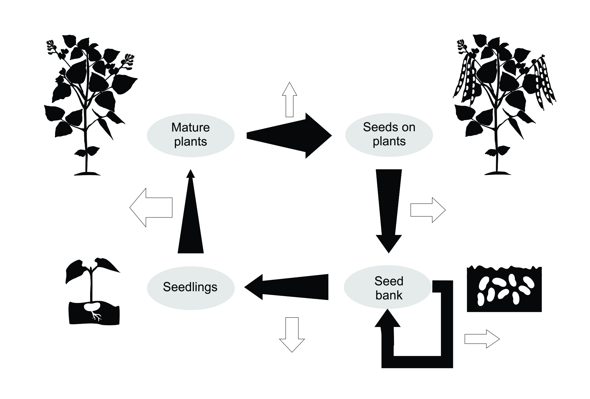
Figure 8.1 Flow chart illustrating the life-cycle of an annual plant (modified from Cousens et al. 1986). Solid arrows indicate the number of individuals at each stage (expanding arrows indicate reproduction; contracting arrows are the result of losses). Open arrows show losses due to various processes, including consumption, disease, germination, dispersal and density-dependent mortality.

In species with overlapping generations, it is common to elaborate the model so that probabilities are a function of the ages, the sizes or the sexes of the individuals. Since we must then keep track of the numbers in each of these classes, we end up with a matrix of probabilities for each step rather than a single value. Typically, the probabilities are expressed via equations, for example relating fecundity in some way to abundance (i.e. density dependence) of the focal species or relating survival to some extrinsic variable such as rainfall. Thus, we end up with a set of equations connected by simple rules and a set of parameters to which we need to ascribe values.

In a spatial model, we must also include probabilities for immigration and emigration and we can make demographic parameters spatially explicit, perhaps based on spatial variation in habitat characteristics. In principle, there is no limit to the complexity that we can introduce into one of these models.

At this point, we are faced with three problems: which drivers do we include? How do we include them (what equations should we use)? And what are appropriate values for the parameters?

8.4.1 Which drivers are important for prediction?

It is intuitive to think that gaining a mechanistic understanding of a system will allow us to achieve better forecasts and thereby make better management decisions. However appealing that logic is, it is not always true and should be evaluated on a case-by-case basis. In ecological forecasting, data limitation is often a problem; and it is more important to achieve reliable predictions within acceptable tolerances, for which very simplistic methods may be adequate, than to include elaborate mathematics and a multitude of interacting variables for which the relevant data are scarce. And even if the model contains all the important mechanisms, it could be highly sensitive to the data (as in chaos theory).

An important example showing that accurate forecasts can be achieved with a basic knowledge of mechanisms comes from atmospheric science, where the art of prediction is much better developed than in ecology. Edward Lorenz (1963) published a system of three ordinary differential equations, designed to be a simplified model of atmospheric flows. He found that any change, no matter how small, in the initial system state led to vastly different forecasts. The system is now known as the Lorenz attractor and spurred the growth of chaos theory. While Lorenz’s conclusion was that long-term weather forecasting is impossible, it also proves that a perfect mechanistic understanding of a system is not enough to make accurate forecasts. While weather forecasts may seem removed from forecasts of organism abundance, the principles of chaos theory have shown that accurate forecasts of fish abundance may be attainable without a deep mechanistic understanding of underlying biotic and abiotic drivers (Perretti et al. 2013; Ye et al. 2015).

In practice, it is the data we have available that decide how mechanistic our models can be. The past decade of ecological research has been driven by the practice of model selection, either hypothesis driven (testing the effects of specific drivers using, for instance, regularisation) or data driven (selecting the most parsimonious model structures among several candidate models by removing parameters) (Hooten and Hobbs 2015). This practice determines the significance of certain drivers, but most frameworks have also been designed to avoid over-parameterisation, that is, fitting and choosing models that are too complex for the data at hand. For instance, if we only have 15 years of abundance data, it is unlikely that we can assess non-linear effects or interactions among climate variables on abundance. Otherwise, we run the risk of inaccurate predictions and especially of extrapolation error.

Beyond being able to predict or forecast, we may want to understand why we see certain patterns within empirical data. For instance, sophisticated methods now exist to use intrinsic properties of abundance time series to forecast future changes in abundances with acceptable accuracy and precision (Pennekamp et al. 2019). Inevitably, when discussing such projected changes, researchers must at least speculate about the mechanisms. Are decreases in survival the culprit? Is lower survival perhaps compensated by reproduction? Are spatial differences in abundance changes due to different responses to a common factor or different underlying factors? Understanding such mechanisms can provide a way to model various scenarios of potential responses of populations to environmental change.

One key source of variation in abundance is the effect of abiotic variables on demographic rates. So, which variables should we include in our models? Sophisticated methods now exist to link variation in survival, reproduction and movement to extrinsic conditions such as weather, soil conditions, or disturbances (e.g. Pedersen et al. 2019). However, even if such variables explain much of the past variation in demographic rates, forecasts are only as robust as (1) our predictions of future values of the abiotic variable itself and (2) our ability to extrapolate responses in response to future abiotic conditions. For instance, if fires are projected to double in intensity in the future, our forecasts of effects on abundances will be more precise if we had captured population responses to high-intensity fires in the past instead of ‘blindly’ extrapolating.

Our ability to accurately specify the relationship between demography and one or more environmental variables will depend on issues such as:

• Omitted variable bias. Some important drivers may be missed altogether by the researcher. There may be little a priori information on which to base variable choice and data might be entirely lacking for many variables. So, we make arbitrary choices based on what is available.

• Relevance of the variable. Although data on some variables may be readily available, they may be of limited use, such as when they are crude surrogates for the true driver, or where they are combinations of many different processes, such as biomass.

• Data quality and extent. Some data may be heavily affected by measurement error, while other data may have limited numbers of observations. Short time series or data collected in remarkably benign periods may fail to have a signal strong enough to be detected.

• Strength of the causal relationship. We need to select variables in terms of their impact on abundance. Although statistical significance is often used as an indicator of the importance of variables, this can be misleading: even weak drivers can be significant if enough measurements are made.

• Correlation with unobserved predictor variables. Many variables may be involved in driving the dynamics of a population, but we may only have data on one or two of them. El Niño events, for example, are typified by changes in rainfall and fire incidence on land, and changes in ocean currents. Extremely low continent-wide winter temperatures are accompanied by periods of reduced river flow followed by extreme discharge as snow and ice melt, with consequent effects on salinity in estuaries and changes in nearshore currents.

An example of how difficult it is to determine the drivers of demography again comes from fisheries. A huge amount of effort is put into the collection of fisheries data in order to inform management decisions. Although there is little that the fishing industry can do to cope with variation in recruitment – other than taking this into account when later setting quotas – there has been a great deal of interest in explaining sources of this variation.

Shepherd et al. (1984) reviewed 47 studies that reported significant correlations with environmental variables, including temperature, salinity (or a surrogate, the inverse of rainfall), wind speed, pressure gradients, upwelling, river discharge and various other proxies (including tree ring width), as well as nine of their own data sets. When re-tested by Myers (1998), around half the correlations were not supported. Myers noted also that there would have been many non-significant correlations generated by researchers that never would have been reported, so the ability to statistically explain variation in fish stock recruitment is much lower than a meta-analysis of published studies would show. The only consistent signal was that correlations with temperature tended to be significant in cases where the species were towards the northern or southern limit of their ranges. It was also notable that there were no significant correlations with the environment for the most intensively studied fisheries (the North Sea and Georges Bank).

Thus far in this section we have considered only extrinsic variables. An important component of many population models is intrinsic population regulation. Not only is this in recognition that abundance (of the focal species or of other species at the same or different trophic levels) is likely to affect demography, but it stops the model from predicting unrealistically high levels of abundance. The way that density dependence is incorporated into population models is based on a variety of well-established relationships, typically either exponential or hyperbolic functions and usually with asymptotic behaviour.

Different branches of ecological research may, for historical reasons, choose particular equations, such as the Beverton and Holt (1957) and Ricker (1975) ‘stock and recruitment’ functions in fisheries. The parameters required for more complex forms of density dependence, such as power terms, can unfortunately be difficult to confidently estimate from empirical data.

Although developing robust predictive models that account for both abiotic and biotic mechanisms in parameterising and projecting demographic rates is difficult, examples exist and show the opportunities and challenges of such approaches. Here we describe just one of them.

Case study 3: meerkat abundance. Kalahari meerkats (Suricata suricatta), social mongooses, have been studied in South Africa since 1993 as part of the Kalahari Meerkat Project. As a result, weekly phenotypic trait (body mass) and demographic data on over 3,000 individuals are currently available, an ideal basis to develop mechanistic forecasting approaches and projections (Clutton-Brock et al. 2016). The meerkats live in a harsh desert climate and have adapted an effective strategy to deal with unpredictable fluctuations in rainfall: cooperative breeding. Only the dominant female reproduces and her young are co-reared by nonbreeding helpers, typically related to the dominant female. This interesting social system is the reason that meerkats have been studied for so long. However, over the years, it has become evident that meerkats, as well as other arid environment specialists, are facing an increasing frequency of temperature extremes under climate change (Bourne et al. 2020). Recent work on meerkats has therefore repurposed the detailed individual data to assess the demographic mechanisms of meerkats’ population responses to ongoing climate change.

The first step in linking trait and demographic data of meerkats to abiotic (temperature and rainfall) and biotic drivers (density and group size) was to parameterise models that allowed the assessment of non-linear effects of different variables and their interactions on body mass change, survival, reproduction and dispersal. Such state-of-the-art modelling approaches offer flexible tools to describe non-linearities inherent in biological data, and their ‘flexibility’ of response curves can be adjusted depending on how much data are available for model fitting. GAMs (generalised additive models) provided good fit to observed variation in meerkat demography and abundances (Paniw et al. 2019). Although the effects on outputs of various sources of uncertainty in the underlying data (such as body mass) were assessed, uncertainty in climatic variables when fitting demographic-rate models was not considered (but was accounted for in projections). Uncertainty in derived climate indices is usually ignored, despite the fact that weather stations in remote areas are sparse and interpolation results in considerable uncertainty.

Once demographic rates were parameterised, population models for meerkats could be built and projected. Because climate variables were included into the GAMs, determining demographic rates, the fate of meerkats under IPCC climate change scenarios could be investigated. This showed that climate change could result in elevated local extinction risk. Their models allowed researchers to propagate various sources of uncertainty in projections, including uncertainty in climate change models. A challenge of such projections is typically that local or regional climatic data are used to parameterize the demographic models while global climate change indices are used for projections, thus creating mismatches in scale. There are ways to alleviate this issue, for instance, using probabilistic forecasting (Fronzek et al. 2010), but no solution is completely satisfactory.

The accuracy of predictions and projections can be assessed by using a training data set for model parameterisation and a separate test data set for validation. Although this approach is ideal, such partitioning of data is not always practical in biological time series. The meerkats are a prime example: despite having over 25 years of continuous data collection, the effects of climate change on meerkats are best understood when modelling the entire time series. This is because the most dramatic effects have occurred in the past eight years, where increases in temperature extremes were accompanied by increases in disease outbreaks, decimating meerkat groups and putting the population at serious risk of extinction (Paniw et al. 2022). These indirect effects of climate change are therefore lagged as, in the case of diseased meerkats, individuals take some time to die. Removing some of the critical years (where disease outbreaks increased) for model validation therefore comes at a loss of power for model fitting whereas hindcasting (using past years for model validation) may not be appropriate as climate-disease interactions were rare. Thus, paradoxically, as the collection of long-term data in meerkats allowed researchers to understand some key mechanisms of climate change effects on an arid environment specialist, validating the likelihood of these mechanisms to bring about a local population collapse will require even more data collection. This is, of course, not a desirable scenario for most management interventions.

Despite the challenges of validating mechanistic models, the meerkat study system is also a fantastic example of the opportunities that understanding these mechanisms bring to ecological research and management. The detailed demographic models in meerkats have been able to demonstrate that the relevant aspects of climate are not just the average annual or seasonal temperatures or precipitation. The timing of climate extremes matters as much as the nature of the extremes, for meerkats and likely most other species (Li et al. 2021).

For the meerkats, under variable rainfall patterns that do not necessarily decrease in the future, higher temperatures may benefit individuals if they occur in the rainy but typically colder season. But if temperatures increase in the hot and dry season, they can bring about dramatic weight loss in individuals which then affects reproductive output further on. Weight loss is stressful and may also exacerbate the risks of deadly infections from endemic diseases (tuberculosis in the case of meerkats). Most social species carry endemic diseases, so that climate change potentially altering disease dynamics is therefore of concern for a wide range of taxa (Plowright et al. 2008; Russell et al. 2020). A better understanding of the mechanisms that affect population dynamics therefore allows us to discuss different ‘what-if’ scenarios beyond specific case studies.

8.5 Model parameterisation and validation

If we have sufficient knowledge, then we can put together a complex model. If we have the resources, then we can obtain good estimates of many parameters. We can expect to achieve good accuracy and precision of our predictions. If we invest further resources, then we might expect further precision and accuracy.

But there is a limit. Every system has what can be referred to as its ‘intrinsic predictive ability’ (Pennekamp et al. 2019) and no matter how much we try, we will never be able to keep making significant improvements to our predictions. An analogy might be the rate at which the world 100 m running record is improved. The trouble is knowing where the limit for population prediction is. In a practical sense, we also run the risk that increases in model complexity will outstrip our ability to estimate the parameters. Model complexity and ‘parameterisation’, as the attribution of values to parameters is called, is always a compromise and it always has the potential to affect the quality of predictions. However, complexity is not always necessary.

COVID-19 modelling provides an example of how we can use models to inform policy without modelling the entire system. The objective of one particular study (Baker et al. 2021) was to explore how polymerase chain reaction (PCR) tests can reduce disease spread at a population level. One approach would be to model the full system, by implementing a PCR testing model within a disease transmission model with multiple disease classes (susceptible, exposed, infectious) and parameterisation of human behaviours regarding mixing and testing, and so on. While theoretically feasible, that model would be quite complex and, from experience, data to estimate parameters would not exist, or, at best, be hard to access.

Detailed mechanistic models not only require a lot of data to parameterise them, but they can also give inaccurate predictions. Accuracy on known data does not give guarantee of accuracy under all other possible actions (Boettiger 2022; Geary et al. 2020). Instead, by framing the question as ‘what reduction in COVID-19 transmission do we get from a given strategy’, a simpler question was posed – one from which we can get important insights without modelling the entire system in detail. Thus, rather than using a large mechanistic model that directly included all the complexities of disease transmission and human testing behaviour, a model of the testing system was developed with relatively simple onward transmission, focusing on important parameters involving laboratory testing capacity and surge testing capacity. Using this model, the COVID-19 researchers produced exemplar scenarios, showing that more testing is not always better if laboratories are overwhelmed.

Model structure and the drivers and the values of the parameters that we include in it will determine the quality of our predictions. In many instances, we use simple models because our ecological knowledge is limited and our estimates of the parameters are weak. But this is one of the important reasons for using models.

We may not want – or expect to achieve – accurate predictions of the abundance of species X at some specified future date. Instead, we want to see what our limited knowledge can tell us about what might plausibly happen: perhaps whether the population is likely to increase, decrease or remain roughly the same or how much impact some environmental perturbation might be expected to have. Many management decisions must be made with incomplete and uncertain information (Burgman et al. 2005). We cannot defer decisions on an endangered species because we do not know enough: we may never know enough and/or we cannot conduct the experiments needed to get better knowledge. So, we make our best attempt. We may guess at some parameters, or ‘borrow’ them from other species. Simple predictions of this type have been used, for example, to determine the ways that we can manage crops to minimise pest resistance (Holst et al. 2007).

How do we assess the quality or the reliability of our predictions? This is usually referred to as model ‘validation’. If our predictions involve time trends of abundance, then strictly speaking we would need an independent and appropriate time series with which to compare our forecasts. The prediction error is then the difference between the observed abundance and the prediction. We must take into account the fact that both the observed and the predicted have error associated with them – in other words, we must partition the contribution of different sources of uncertainty to our metrics of interest (Petchey et al. 2015). We do not know the actual abundance, we just have an estimate of it that may be quite crude. And although it is rarely calculated, our predictions involve errors due to the estimates of the parameters and the structure of the model. One way of addressing the precision of the model’s predictions is to use a Monte Carlo simulation: we can do multiple runs of the model, with parameter estimates, initial conditions and drivers taken from a frequency distribution based on the raw data used for parameter estimation. We can even use prior knowledge to help us estimate parameters and their uncertainty, undoubtedly an important reason for the popularity of Bayesian methods in applied ecology. We might even have situations where the precision of the prediction is good, but accuracy of prediction might be very poor because we have failed to identify bias or because the model is structurally unsound.

The lack of appropriate validation data is a common hurdle in population modelling. For a scenario prediction, we often speculate about the amount by which a given parameter might change; this may be informed by evidence or it may be a ‘ball-park’ guess. For example, we might say ‘suppose hunting causes a 50% reduction in male survival’, something that we put out there for the sake of argument, when we actually have no idea. A rigorous test of a model prediction would need data that have been assembled under those specific scenarios. But we do not have such data, because those scenarios have never occurred and have never been included in an experiment.

In cases such as climate change, we cannot validate our predictions of the future until those changes have happened – though we could test it to some degree retrospectively on older time series. We must, therefore, treat scenario predictions and projections with an appropriate degree of caution. No matter how complex the model, we have made no more than a best guess and we must be honest about this and communicate the uncertainties in the model and in the forecasts.

Model validation is important and is often stressed in introductory materials about modelling. In practice, it has traditionally been overlooked in many modelling papers because the appropriate data are too often lacking. A prediction is made and validation must wait until someone comes along in the future. Many models, however, are never really complete and validation, model development and the collection of new data go hand in hand. The model is never finished, it is constantly under review and its predictions are – we hope – constantly improving. We know the predictions have some error, whether we can measure it or not, but through sustained effort that error will continue to fall. This process has been formalised with the term ‘iterative near-term forecasting’ (analogous to the ideas of adaptive management and rapid prototyping) (Dietze et al. 2018).

It is self-evident that if we want a high level of precision and accuracy, then we will need to invest adequate resources into assembling the information needed.

We take it for granted that in every modelling project there will be care taken to generate the best estimates of parameters that we can from the data that we have on hand. As we have indicated elsewhere in this chapter, we glean parameter values from a range of sources. These may include long-term demographic studies with intensive monitoring, large sample sizes and extensive data sets: i.e. high-quality data that would make most modellers’ mouths water! We spend a great deal of effort in using state-of-the-art methods to obtain the best estimates of our parameters; there is a great deal of literature on these methods. But parameter estimates also include data from short-term studies (perhaps graduate theses), means reported in (or calculated from) published papers, unreplicated observations and expert opinion (best guesses).

We know that parameterisation of models is crucial to model performance, yet we often take what we can get, publish the results and reflect on the predictions made from a job well done. Some studies, particularly well-funded long-term studies of iconic species, do put a great deal of effort into further research to improve parameter estimates. However, increasing accuracy and precision requires effort and investment that may be better utilised elsewhere.

In predictive modelling, we should more frequently ask ‘how much investment is additional parameter improvement worth?’, and ‘which parameters justify the greatest research effort?’. We can perform sensitivity analyses for any model, altering the values of each parameter systematically and then observing the incremental impact on the quantity predicted (in our case population abundance).

Linear models of simple life histories are often examined using elasticity metrics, while sensitivity analyses have also been developed for ‘Bayesian belief networks’. We will say more about this when we discuss ‘value of information’ analysis later. And however simple or complex the population model is, we still need to conduct optimisation to find the best management strategy (optimisation methods have their own entire field, which we won’t talk about here).

8.6 From forecasts to policy

So far, this chapter has explored models of population dynamics and using them to make predictions. But what do we do with a model once we have it? Apart from using models to improve our fundamental understanding of species, we can use them to improve management decisions. There is an entire area of research ‘decision science’ devoted to the study of making decisions (Box 8.1).

The use of decision science in ecology has increased particularly over the last decade: some prominent examples include spatial planning for conservation (Ball et al. 2009) and the Project Prioritization Protocol for targeting and prioritising investment in threatened species (Joseph et al. 2009).

In management contexts, predictions fall into three broad categories: nowcasting, forecasting and scenario analysis. All play a role in management, but they are used in very different ways. ‘Nowcasting’ is about estimating the current state of a system from observations. As defined earlier in the chapter, ‘forecasting’ is predicting the future state of a system, given current knowledge, while ‘scenario analysis’ is about modelling a range of potential future management options and/or across a range of plausible, but uncertain, model parameters.

There are two broad types of decision-making questions we may seek to answer with mathematical models. The first is ‘do we need to act?’ And the second is ‘what action should we take?’ The types of models required for the former are nowcasts and forecasts, while the latter is typically done with scenario analysis (which may be built on, or incorporate, nowcasts and forecasts). When using these modelling tools in a decision-making framework, we need to think carefully about how models will be used within the decision-making process. Models are often designed to answer specific types of questions and, if those questions do not align with the decisions being made, then the potential for impact of that model in the decision-making process will be limited.

Box 8.1 What is decision science?

While we do not provide a detailed guide to decision science here (instead, see Hemming et al. 2021), we provide a brief description to enable discussion of modelling. The process of framing problems by focussing on the objectives and actions, rather than on fundamental science, is key to the decision science approach to solving problems. Beyond specifically helping people to make decisions, another important use of the approach is in helping with questions about model complexity. It is easy to make models more complex to try to capture more realism; however, as we have mentioned elsewhere in this chapter, it is difficult to determine how much complexity is enough. While we cannot resolve this issue in general, decision science allows us to ask the related question: ‘how much complexity do I need to make a useful model to inform my current decision?’

Central to the approach is a structured decision-making workflow. Broadly, the steps are:

1. Set management objectives and performance measures.

2. Decide on potential actions, which includes ‘no action’.

3. Estimate consequences of different actions on the objective.

4. Evaluate trade-offs.

5. Make the decision.

In a fully-fledged structured decision-making workshop, researchers can guide stakeholders through the entire structure of the decision-making process. However, addressing every point in the structured decision-making process is not necessary for it to be a useful concept for all scientists trying to make a policy impact with science. The key role of population modelling is at step 3 – to estimate how different actions will affect a system and our management objectives. Note that uncertainties are inherent in decision-making (Milner-Gulland and Shea, 2017), though it is possible that the decision will remain the same even if uncertainties are resolved (see the discussion on value of information later in the chapter). Quantifying the uncertainties in the subsequent population model (such as providing credible intervals) can reveal actions that are robust to the remaining uncertainties.

In recent years, there has been an increasing number of papers modelling population dynamics with species interaction to predict potential management outcomes (e.g. Baker et al. 2017). However, in terms of direct impact to policy, one of the most recent applications of decision science with wide-ranging impact is the National Plan for COVID-19 Modelling in Australia (Doherty Institute, 2021). In this study, modelling was used to advise the Australian Government on potential policies, steps and actions to bring Australia out of lockdown due to the COVID-19 pandemic. This model provides an interesting case study, because it is purely focused on step 3, estimating consequences, and not the entire structured decision-making workflow. Awareness of the other steps was critical to ensure that the correct questions were being answered.

 

When creating models to inform management, we face different criteria for what makes a good model. Often in ecology we are concerned about making accurate and precise predictions of populations into the future. However, in a decision-making setting, our aim is to correctly distinguish between a set of management options and select the truly best option, and not to make our models maximally accurate and precise per se. The accuracy and precision required depend on the question being asked, who is asking it and how it is being asked.

Aside from the ‘standard’ structured decision-making process (Box 8.1), there are a range of other techniques that fall under the decision science umbrella. Two particularly important concepts are ‘adaptive management’ and ‘value of information’ theory. Adaptive management is in some ways an extension of structured decision-making (Walters and Holling 1990), where decisions are made regularly with updated information (for example, yearly decisions on population control). We can repeat the same decision making process, refining and updating our models each time and learning from past actions as we proceed. Value of information theory focuses on learning about the uncertainties in models and how they affect the outcomes, to determine whether it is worth the resources to acquire more information before making the decision (Canessa et al. 2015). It is related to optimal experimental design, which seeks to determine how to optimally design an experiment to reduce system uncertainty.

In the face of a constantly changing world, our knowledge about ecological systems and our ability to forecast what would happen under various management actions are imperfect. Adaptive management acknowledges this, allowing us to iteratively make improvements rather than decide and keep to a fixed set of actions. It can be the most optimal and cost-effective management scheme (Walters and Holling 1990). In addition to repeating the decision making process regularly, adaptive management also involves monitoring and using that information to inform the next decision-making process. Updating information, data and predictions is key to reducing uncertainties and improving outcomes at each cycle.

To make use of adaptive management, after making and implementing a decision, the results should be monitored. It is important to pick indicators or measurements that can detect the changes in the system when management is changed. Did the results play out as expected or not? During the implementation process, can we uncover more information that could now inform a better decision? The decision-monitoring process of adaptive management allows researchers to test the forecasts of their model on real impacts and measure how robust the original predictions were. Repeating this allows us to thus expand, modify and iteratively correct forecast models, leading to a better understanding of the important factors and major interactions in ecological systems, similar to how weather forecasting has improved over recent decades (Bauer 2015).

There are many specific adaptive management models created for different ecological systems and requirements. A number of proposed frameworks include management strategy evaluation (MSE) (Punt et al. 2016) and strategic adaptive management (SAM: Kingsford et al. 2011). Adaptive management requires strong and continuous communication between multiple parties, from stakeholders, to decision-makers and scientists.

Whether we spend the time or resources to gain more information is itself a decision, but it is not guaranteed that knowing more would lead to a better decision, nor whether the cost of doing more research will lead to a better return on the decision. Eventually, one must stop monitoring and start taking direct actions, lest one ends up ‘monitoring a species until it becomes extinct’ (Lindenmayer et al. 2013). While more information can be tempting, especially to researchers, more research may not be the best action to take: gathering information takes time and resources, delaying a potential management decision and action and potentially allowing the current state of the system to worsen. However, without sufficient information, we are at risk of making uninformed decisions.

Similar to the problem of ‘how complex should the model be’ is the problem ‘how much information do we need?’ Value of information theory is a formal framework that allows us to estimate the cost and return on further information gathering. We can use a model to conduct a value of information analysis, which involves a structured analysis of trade-offs between obtaining more information versus acting with the current available information, and to determine what would be useful information to obtain.

These are not the only frameworks for making decisions. Different ecological and real-world systems contain complexities, and there are a wide range of decision science tools to address them. For example, rapid prototyping can produce quick initial decisions, which are then iteratively improved over a series of small/frequent milestones. There are decision science frameworks for multiple objectives (i.e. multi-criteria decision analysis: Mendoza and Martins 2006).

To ecological complexity must be added the complexity from other humans: decision makers, titleholders and stakeholders. Researchers who are tasked with modelling the ecological system must be in constant communication with these groups as the resulting actions are made by them and will affect them directly (Gibbons et al. 2008). When running forecasts for decision-making, it is important to communicate uncertainty (Baker and Bode 2020) and also to understand how risk-averse the decision-maker is. For example, whether they prefer to minimise the probability of the worst outcome or whether they want to maximise the probability of a good outcome, and so forth. One approach for dealing with risk and uncertainty is ‘stochastic dominance’, which can be used to rank alternative management actions using probability distributions (Canessa et al. 2016). In addition, involving titleholders and stakeholders in the decision-making process can improve the future decision implementation (Bennett et al. 2019). It would not be surprising if decision-makers, titleholders, stakeholders and even the modellers have conflicts. If so, then other methods under decision science might need to be used, such as negotiation theory and conflict resolution.

There are many complexities to consider when it comes to using modelling to make real policy impact. Earlier in the chapter, we mentioned how decision science was used in the context of COVID-19 modelling and PCR testing. To put the above discussion in context, we will now give another example of COVID-19 modelling, as well as a case in which ecological modelling has been used to help inform policy and management decisions for a threatened species.

Case study 4: dynamical population modelling for COVID-19 policy. Writing about modelling and policy in 2023, it is hard not to reflect on the role of modelling for decision-making throughout the COVID-19 pandemic. Rarely – if ever – have mathematical models of biological dynamics featured so prominently in our society. Hence, COVID-19 modelling gives us a range of recent examples of how mathematical modelling has been used to engage with policy. Although this book’s focus is on ecology, we make no apology for using another COVID-19 example. Its topicality will resonate with the reader: both humans and diseases can be studied ecologically (they are both organisms within an environment) and they have populations.

In 2020, COVID-19 spread to Australia, triggering nation-wide lockdowns that successfully prevented the wide destructive spread of the disease. As vaccines were becoming available, in 2021 the Australian Government decided that they wanted to end the lockdowns and re-open borders, which would necessarily mean accepting the spread of COVID-19 through its population. Scientists modelled population and infectious disease dynamics to inform government decisions (Doherty Institute 2021), using a range of models from simple dynamical systems to complex and highly parameterised agent-based formulations. The modelling team’s role was to engage with the Australian Government to understand the objectives and the potential decisions and develop models where they could explore various actions for ending lockdowns since vaccines were finally available for use. The objectives, actions, trade-offs and final decisions (i.e. steps 1, 2, 4 and 5 of the decision-making process in Box 8.1) were all determined by the Australian Government, not by the modellers. Using modelling, the team could simulate the given actions, mapping the outputs to the real-world objectives. The team had a close collaboration with the Department of the Treasury to evaluate various trade-offs, considering the broad impacts of disease spread alongside other metrics, including economic impact of both restrictions and public health impacts (Australian Government 2021). The modelling team ultimately delivered a range of scenarios from which government could choose, depicting how border opening at different thresholds of vaccination coverage would likely affect future infections, disease outcomes and the clinical impacts.

This case study exemplifies that a decision science approach is not only relevant when scientists can provide significant input into each step. By engaging with relevant groups and understanding steps 1, 2, 4 and 5 from their perspective, we can use scientific modelling to inform step 3 (i.e. estimating the consequences of different actions on the objective). If scientific modelling is done without understanding the broader scope of potential actions and objectives, the work may not be usable and may be unable to affect decisions, for example if the considered actions will never be considered realistically (e.g. due to cost) or politically, or the objectives are not actually being considered by the policy makers.

The COVID-19 case study had the benefit of a wealth of data from around the world to inform the models, and hence the subsequent actions. Few programs on important, unique and rare ecological species are in that position! In the next case study, we look at the management of one threatened Australian animal with uncertain information about how it interacts with its threats and how this is now being resolved.

Case study 5: adaptive management of malleefowl. The malleefowl (Leipoa ocellata) is a ground-dwelling bird that builds large mounds to incubate its eggs. It is found across southern Australia and is formally recognised as being endangered. Threats include historical habitat clearance, predation from introduced and native species, and changing fire regimes. The National Malleefowl Recovery Team have been implementing a recovery plan since 1989, working with many other organisations across southern Australia (The National Malleefowl Recovery Team 2022). Nesting activity has been monitored since the 1990s and, at present, a number of different ongoing management activities aim to increase abundance, including fox baiting, fencing and re-vegetation. However, data analysis over time has drawn conflicting conclusions as to whether fox baiting in particular was effective.

Hauser et al. (2019) worked in collaboration with multiple groups such as land managers, experts and many other stakeholders including government agencies, mining companies, traditional owners, farmers, private landholders and leaseholders to facilitate a decision science process (steps 1-5 listed in Box 8.1). They developed an ensemble ecosystem model to predict malleefowl abundance, involving 80 different interactions between 14 different ecological components, including malleefowl density, vegetation density, rainfall quality, rabbit density and fox density. They simulated the five-year consequences of various potential management actions on abundance. The model predicted that management actions targeting disease and inbreeding had a high probability of producing positive effects. In contrast, management action addressing fox predation could lead to both large positive effects in malleefowl abundance and large negative effects in their abundance. In short, there was high uncertainty.

The decision-makers and stakeholders wanted to resolve the uncertainty about the interactions between malleefowl and its predators. Hence, the research team developed a predator control experiment. They also conducted a statistical power analysis to determine how many sites and how long the experiment needed to run in order to resolve the uncertainties. After multiple workshops and the involvement of multiple organisations and groups across Australia, the Adaptive Management Predator Experiment is now in-progress. As part of this experiment, different sites were strategically chosen to either be managed (fox baiting) or purposefully unmanaged (no fox baiting). There are 22 control-treatment paired sites in eight clusters, chosen such that they have similar environmental conditions. The known malleefowl nesting mounds (found in various monitoring efforts) are monitored for activity, as a proxy for abundance (since it is difficult to monitor the malleefowl themselves).

The experiment will run for five years. As part of their experimental plan for learning, the researchers presented statistical methods to evaluate the future results after monitoring, with a model to estimate the effect of fox baiting on malleefowl nesting mounds that can be updated as data come in. It remains to be seen how the malleefowl management will change after this experiment concludes. If decision-makers adjust their management actions in the future, then this would become a rare example of successful adaptive management in biodiversity conservation at a landscape scale. Decision-makers could even embark on a new experiment to resolve other uncertainties relating factors that affect malleefowl abundance.

While there are many examples of adaptive management of natural resources in the context of harvesting, there are few successful implementations in biodiversity conservation for various reasons (Westgate et al. 2013). Biodiversity conservation adaptive management publications tend to be light on the follow-up after the first cycle of the decision-making process. If adaptive management is truly to be implemented, then it is not enough for the research team to meet with the decision-makers and stake-holders to help make one decision; they need to continue the conversation, play a role in updating the models and thus aid decision-makers to adaptively make decisions over time. This requires strong relationships and connections, a difficult human problem that needs to be overcome before one can start working on the ecological problem together, and ongoing access to funds (another difficult problem).

8.7 So what?

In this chapter, we have delved into population models and touched on the numerous aspects that affect their accuracy and reliability. Predictive modelling is an extremely important part of empirical ecology, requiring sufficient expertise and resources. The availability of user-friendly software has made predictive modelling much more accessible, but it can be misused in the wrong hands.

We have considered how predictions should be based, where possible, on sound empirical data and should be revised upon new information. Researchers need to consider not just whether more empirical data are needed, but what data and why. Although there has been a tendency among ecologists to believe that more research will serendipitously result in better insights into management options, this is not necessarily the case, and some types of research are more useful than others.

Regardless of how and what model ecologists ultimately choose for their context and purpose, there will always be limitations and uncertainty. A detailed understanding of fundamental ecology often helps us to model, especially when we have limited data. But we also note that in many situations, such as policy impact, high precision and accuracy may not be necessary, and that it is much more important to have good predictions for broad scenarios targeted towards well-defined objectives in a decision science framework. Prediction is both a way to demonstrate scientific understanding about scientific theories, and also what we can use to make scientifically rigorous decisions to positively change the world around us.

Historically, empirical ecology has largely consisted of case studies of numerous species and corresponding population models, representing isolated or small systems as they are right now. However, with increasingly many challenges facing the ecological landscape and species worldwide, we need ecological forecasting to predict what may happen in the future and to explore how we can prevent negative outcomes and ensure maximum benefits under alternative scenarios.

In other disciplines, such as economics, engineering, or climatology, generalisable outcomes of studies are used as reliable indicators of future trends. Can we achieve this in ecology? Or is ecology simply too complex? Or perhaps, are the assumptions in other disciplines simply not complex enough? Answering these questions will likely determine the future of ecological research because in order to be taken seriously, ecologists need to show confidence in their forecasting ability to mitigate emerging global threats. The first step towards this goal would require us to propose generalisable rules for predictions. But how do we want to achieve this? Is the future to work on even more local case studies and generalise from these, - as has been done for life history theory? How many such studies are needed: or is the need unbounded? Every ecosystem, community or population needs case-specific data, to help formulate models and to test them. Or is global large-scale research the way to go (such as DroughtNet: Sevilleta 2022)? There are trade-offs in relation to scale. Local studies are more equitable, but produce a lot of noise. Global approaches may produce too little noise and tend to be exclusionary. In short, there is no one-approach-fits-all method when it comes to ecological forecasting.

We currently have a wide range of techniques that allow us to model just about whatever we want, and many more are under development. Theoretical model complexity itself is now only constrained by computational power. However, this comes at the cost of uncertainty or high data requirements to parameterise and calibrate a model to reflect the current known ecological status. Furthermore, there is no guarantee that a complex model will do any better than a simple model at predicting what is unknown. Even if a model can successfully predict the outcome of one ecological action, it may be completely wrong about the outcomes from other ecological actions.

For each situation, researchers must carefully choose which predictive or forecasting models are most suitable for their context. There is no easy way to do this. The end use of the model, what it is that we want to achieve, should dictate much of what we do.

In the case of fundamental ecological research designed to extend our basic understanding, it is a difficult question to answer what the biggest goals are. We delve ever deeper into the details of every issue. Others before us have argued that any further developments in theoretical ecological modelling need to go hand in hand with research that aims to test not just their qualitative predictions (Simberloff 1981; Haller 2014), but also the assumptions they make and the processes that were incorporated. But as we have seen in the case of predator-prey cycles, testing may be difficult and illusory.

For applied ecology, the situation might be quite different. There may be a plethora of contexts and objectives, but the use of structured methods and processes within decision science can help enormously. There are methods to help to better establish what we truly want to achieve, identifying what the constraints to decisions are, guiding us to options and evaluating what the trade-offs are in their implementation. Decision science can help considerably in this way and is better than trying to make decisions purely by instinct.

So, should every ecologist become a decision scientist? No! Although some funding agencies are urging researchers towards more applied outcomes, there is no requirement for every ecologist to do work that has a clear path from research to impact. However, for anyone who wants to impact decision-making and policy, decision science provides a useful perspective to better understand how to contribute.

For some, that engagement may be running structured decision-making workshops and working through each step of the decision-making process with relevant stakeholders. For others, it may focus solely on improving how we model systems, so we can better estimate the consequences of actions. And for some, it could be investigating the fundamental building blocks of ecosystems, enabling better modelling in the future. For this final group, the use of the decision science perspective is not about solving problems directly, but as an aid in understanding what fundamental mechanisms are critical to understand in order to facilitate better decision-making in the future.

There is no universal correct answer for what type of work to do, there is only what is right for each project.

8.8 References

Australian Government. 2021. Economic impact analysis: National plan to transition to Australia’s national COVID-19 response. https://treasury.gov.au/publication/p2021-196731 accessed 17 August 2022.

Baker C. M., I. Chades, J. McVernon, A. P. Robinson, and H. Bondell. 2021. Optimal allocation of PCR tests to minimise disease transmission through contact tracing and quarantine. Epidemics 37:100503. doi:10.1016/j.epidem.2021.100503

Baker, C. M., and M. Bode. 2020. Recent advances of quantitative modeling to support invasive species eradication on islands. Conservation Science and Practice 3:e246. doi:10.1111/csp2.246

Baker, C.M., A. Gordon, and M. Bode. 2017. Ensemble ecosystem modeling for predicting ecosystem response to predator reintroduction. Conservation Biology 31:376-384. doi:10.1111/cobi.12798

Ball, I.R., H. P. Possingham, and M. E. Watts. 2009. Marxan and relatives: Software for spatial conservation prioritization. In Spatial conservation prioritization: quantitative methods and computational tools, eds A. Moilanen, K. A. Wilson, and H. P. Possingham, 185–195. New York: Oxford University Press.

Bauer, P., A. Thorpe, and G. Brunet. 2015. The quiet revolution of numerical weather prediction. Nature 525:47-55. doi:10.1038/nature14956

Bennett, N. J., A. Di Franco, A. Calò, et al. 2019. Local support for conservation is associated with perceptions of good governance, social impacts, and ecological effectiveness. Conservation Letters 12:e12640. doi:10.1111/conl.12640

Beverton, R. J. H.; and S. J. Holt. 1957. On the dynamics of exploited fish populations. Fishery Investigations Series II Volume XIX, Ministry of Agriculture, Fisheries and Food.

Blasius, B., L. Rudolf, G. Weithoff, U. Gaedke, and G. F. Fussmann. 2020. Long-term cyclic persistence in an experimental predator–prey system. Nature 577:226–230. doi:10.1038/s41586-019-1857-0

Boettiger, C. 2022. The forecast trap. Ecology Letters 25:1655-1664. doi:10.1111/ele.14024

Bolker, B. 2004. Continuous-space models for population dynamics. In Ecology, genetics, and evolution of metapopulations, eds I. Hanski, and O. E. Gaggioti, 45-69. San Diego: Elsevier Science.

Bourne, A. R., J. J. Cunningham, C. N. Spottiswoode, and A. R. Ridley. 2020. Hot droughts compromise interannual survival across all group sizes in a cooperatively breeding bird. Ecology Letters 23:1776–1788. doi:10.1111/ele.13604

Bronowski, J. 1979. The origins of knowledge and imagination. New Haven: Yale University Press.

Burgman, M. A., D. B. Lindenmayer, and J. Elith. 2005. Managing landscapes for conservation under uncertainty. Ecology 86:2007-2017. doi:10.1890/04-0906

Canessa, S., G. Guillera-Arroita, J. J. Lahoz-Monfort, et al. 2015. When do we need more data? A primer on calculating the value of information for applied ecologists. Methods in Ecology and Evolution 6:1219-1228. doi:10.1111/2041-210X.12423

Canessa, S., J. G. Ewen, M. West, M. A. McCarthy, and T. V. Walshe 2016. Stochastic dominance to account for uncertainty and risk in conservation decisions. Conservation Letters 9:260-266. doi:10.1111/conl.12218

Caswell, H. 1988. Theory and models in ecology: A different perspective. Ecological Modelling 43:33-44.

Clark, J. S. 1998. Why trees migrate so fast: Confronting theory with dispersal biology and the paleorecord. American Naturalist 152:204-224.

Clark, J. S., C. Fastie, G. Hurtt, et al. 1998. Reid’s paradox of rapid plant migration: Dispersal theory and interpretation of paleoecological records. BioScience 48:13-24.

Clutton-Brock, T. H., and M. Manser. 2016. Meerkats: Cooperative breeding in the Kalahari. In Cooperative breeding in vertebrates: Studies of ecology, evolution, eds W. D. Koenig, and J. L. Dickinson, 294–317. Cambridge: Cambridge University Press. doi:10.1017/CBO9781107338357.018

Cousens, R., C. J. Doyle, B. J. Wilson, and G. W. Cussans. 1986. Modelling the economics of controlling Avena fatua in winter wheat. Pesticide Science 17:1-12.

Cousens, R., C. Dytham, and R. Law. 2008. Dispersal in plants: A population perspective. Oxford: Oxford University Press. doi:10.1111/j.1095-8339.2012.01210.x

Dayton, P. K. 1979. Ecology: A science and a religion. In Ecological processes in coastal and marine systems, ed. R. J. Livingstone, 3-18. New York: Plenum Press.

Dietze, M. C., A. Fox, L. M. Beck-Johnson, et al. 2018. Iterative near-term ecological forecasting: Needs, opportunities, and challenges. Proceedings of the National Academy of Sciences of the United States of America 115:1424-1432. doi:10.1073/pnas.171023111

Doherty Institute. 2021. Doherty Institute modelling report for national cabinet. https://www.doherty.edu.au/news-events/news/doherty-institute-modelling-report-for-national-cabinet accessed 16 August 2022

Fisher, R. A. 1937. The wave of advance of advantageous genes. Annals of Eugenics 7:355-369.

Fronzek, S., T. R. Carter, J. Räisänen, L. Ruokolainen, and M. Luoto. 2010. Applying probabilistic projections of climate change with impact models: a case study for sub-Arctic palsa mires in Fennoscandia. Climatic Change 99:515–534. doi:10.1007/s10584-009-9679-y

Geary, W.L., M. Bode, T. S. Doherty, et al. 2020. A guide to ecosystem models and their environmental applications. Nature Ecology and Evolution 4:1459–1471. doi:10.1038/s41559-020-01298-8

Gibbons, P., C. Zammit, K. Youngentob, et al. 2008. Some practical suggestions for improving engagement between researchers and policy-makers in natural resource management. Ecological Management and Restoration 9:182-186. doi:10.1111/j.1442-8903.2008.00416.x

Gustafsson, L., and M. Sternad. 2016. A guide to population modelling for simulation. Open Journal of Modelling and Simulation 4:55-92. doi:10.4236/ojmsi.2016.42007

Haller, B. C. 2014. Theoretical and empirical perspectives in ecology and evolution: A survey. BioScience 64:907–916. doi:10.1093/biosci/biu131

Hastings, A. 2020. Long-term predator-prey cycles finally achieved in the lab. Nature 577:172-173. doi:10.1038/d41586-019-03603-3

Hauser, C. E., D. Southwell, J. J. Lahoz-Monfort, et al. 2019. Adaptive management informs conservation and monitoring of Australia’s threatened malleefowl. Biological Conservation 233:31-40. doi:10.1016/j.biocon.2019.02.015

Hefley, T. J., M. B. Hooten, R. E. Russell, D. P. Walsh and J. A, Powell. 2017. When mechanism matters: Bayesian forecasting using models of ecological diffusion. Ecology Letters 20:640-650. doi:10.1111/ele.12763

Hemming, V., A. E. Camaclang, M. S. Adams, et al. 2021. An introduction to decision science for conservation. Conservation Biology 36:e13868. doi:10.1111/cobi.13868

Holst, N., I. A. Rasmussen, and L. Bastiaans. 2007. Field weed population dynamics: A review of model approaches and applications. Weed Research 47:1-14. doi:10.1111/j.1365-3180.2007.00534.x

Houlahan, J. E., S. T. McKinney, T. M. Anderson, and B. J. McGill. 2017. The priority of prediction in ecological understanding. Oikos 126:1-7. doi:10.1111/oik.03726

Hooten, M. B., and Hobbs, N. T. 2015. A guide to Bayesian model selection for ecologists. Ecological Monographs 85:3-28. doi:10.1890/14-0661.1

Hurrell, J. W. 1995. Decadal trends in the North Atlantic Oscillation: regional temperatures and precipitation. Science 269:676–679.

Joseph, L.N., R. F. Maloney, and H. P. Possingham. 2009. Optimal allocation of resources among threatened species: a Project Prioritization Protocol. Conservation Biology 23:328–338. doi:10.1111/j.1523-1739.2008.01124.x

Kingsford, R. T., H. C. Biggs, and S. R. Pollard. 2011. Strategic adaptive management in freshwater protected areas and their rivers. Biological Conservation 144:1194-1203. doi:10.1016/j.biocon.2010.09.022

Kolmogorov, A., I. Petrovskii, and N. Piskunov. 1937. Study of a diffusion equation that is related to the growth of a quality of matter and its application to a biological problem. Moscow University Mathematics Bulletin 1:1-26.

Krebs, C. J. 2002. Beyond population regulation and limitation. Wildlife Research 29:1-10. doi:10.1071/WR01074

Krebs, C. J., R. Boonstra, and S. Boutin. 2018. Using experimentation to understand the 10-year snowshoe hare cycle in the boreal forest of North America. Journal of Animal Ecology 87:87-100. doi:10.1111/1365-2656.12720

Krebs, C. J., R. Boonstra, S. Boutin, and A. R. E. Sinclair. 2001. What drives the 10-year cycle of snowshoe hares? BioScience 51:25-35. doi:10.1641/0006-3568(2001)051[0025:WDTYCO]2.0.CO;2

Lele, S. R., and K. L. Allen. 2006. On using expert opinion in ecological analyses: A frequentist approach. Environmetrics 17:683-704. doi:10.1002/env.786

Levins, R. 1966. The strategy of model building in population biology. American Scientist 54:421-431.

Li, G., X. Wan, B. Yin, et al. 2021. Timing outweighs magnitude of rainfall in shaping population dynamics of a small mammal species in steppe grassland. Proceedings of the National Academy of Sciences of the United States of America 118:e2023691118. doi:10.1073/pnas.2023691118

Lindenmayer, D. B., M. P. Piggott, and B. A. Wintle. 2013. Counting the books while the library burns: why conservation monitoring programs need a plan for action. Frontiers in Ecology and the Environment 11:549-555. doi:10.1890/120220

Lorenz, E. N. 1963. Deterministic nonperiodic flow. Journal of the Atmospheric Sciences 20:130–141.

Lu, C., and B. Zhou. 2018. Influences of the 11-yr sunspot cycle and polar vortex oscillation on observed winter temperature variations in China. Journal of Meteorological Research 32:367–379. doi:10.1007/s13351-018-7101-2

Mendoza, G. A., and H. Martins. 2006. Multi-criteria decision analysis in natural resource management: A critical review of methods and new modelling paradigms. Forest Ecology and Management 230:1-22. doi:10.1016/j.foreco.2006.03.023

Milner-Gulland, E. J., and K. Shea. 2017. Embracing uncertainty in applied ecology. Journal of Applied Ecology 543:2063-2068. doi:10.1111/1365-2664.12887

Myers, R. A. 1998. When do environment-recruitment correlations work? Reviews in Fish Biology and Fisheries 8:285-305

Olden, J. D., J. J. Lawler, and N. L. Poff. 2008. Machine learning methods without tears: A primer for ecologists. The Quarterly Review of Biology 83:171-193. doi:10.1086/587826

Paniw, M., C. Duncan, F. Groenewoud et al. 2022. Higher temperature extremes exacerbate negative disease effects in a social mammal. Nature Climate Change 12:284–290. doi:10.1038/s41558-022-01284-x

Paniw, M., N. Maag, G. Cozzi, T. Clutton-Brock, and A. Ozgul. 2019. Life history responses of meerkats to seasonal changes in extreme environments. Science 363:631–635. doi:10.1126/science.aau5905

Pedersen, E. J., D. L. Miller, G. L. Simpson, and N. Ross. 2019. Hierarchical generalized additive models in ecology: An introduction with mgcv. PeerJ 7:e6876 doi:10.7717/peerj.6876

Peers, M. J. L., Y. N. Majchrzak, A. K. Menzies, et al. 2020. Climate change increases predation risk for a keystone species of the boreal forest. Nature Climate Change 10:1149–1153. doi:10.1038/s41558-020-00908-4

Pennekamp, F., A. C. Iles, J. Garland, et al. 2019. The intrinsic predictability of ecological time series and its potential to guide forecasting Ecological Monographs 89:e01359. doi:10.1002/ecm.1359

Perretti, C.T., S. B. Munch, and G. Sugihara. 2013. Model-free forecasting outperforms the correct mechanistic model for simulated and experimental data. Proceedings of the National Academy of Sciences of the United States of America 110:5253–5257. doi:10.1073/pnas.1216076110

Petchey, O. L., M. Pontarp, T. M. Massie, et al. 2015. The ecological forecast horizon, and examples of its uses and determinants. Ecology Letters 18:597-611. doi:10.1111/ele.12443

Peters, R.F. 1991. A critique for ecology. Cambridge: Cambridge University Press

Plowright, R. K., S. H. Sokolow, M. E. Gorman, P. Daszak, and J. E. Foley. 2008. Causal inference in disease ecology: investigating ecological drivers of disease emergence. Frontiers in Ecology and the Environment 6:420–429. doi:10.1890/070086

Punt, A. E., D. S. Butterworth, C. L. de Moor, J. A. De Oliveira, and M. Haddon. 2016. Management strategy evaluation: Best practices. Fish and Fisheries 17:303-334. doi:10.1111/faf.12104

Reid, C. 1899. The origin of the British flora. London: Dulau.

Ricker, W.E. 1975. Computation and interpretation of biological statistics of fish populations. Bulletin of the Fisheries Research Board of Canada 191, Ottawa.

Russell, R., G. V. DiRenzo, J. Szymanski, et al. 2020. Principles and mechanisms of wildlife population persistence in the face of disease. Frontiers in Ecology and Evolution 8:569016. doi:10.3389/fevo.2020.569016

Salguero-Gómez, R. and M. Gamelon (eds). 2021. Demographic methods across the tree of life. Oxford: Oxford University Press.

Sevilleta Long-Term Ecological Research. 2022. https://sevlter.unm.edu/droughtnet-experiment/#:~:text=The%20Drought%20Network%20is%20a,across%20biomes%20and%20climate%20gradients. Accessed 1 September 2022.

Shepherd, J. G., J. G. Pope, and R. D. Cousens. 1984. Variations in fish stocks and hypotheses concerning their links with climate. Rapports et Proces-verbaux des Réunions. Conseil International pour l’Éxploration de la Mer 185:255-267.

Sheriff, M. J., C. J. Krebs, and R. Boonstra. 2011. From process to pattern: How fluctuating predation risk impacts the stress axis of snowshoe hares during the 10-year cycle. Oecologia 166:593-605. doi:10.1007/s00442-011-1907-2

Simberloff, D. 1981. The sick science of ecology. Eidema 1:49–54.

Skellam, J. G. 1951. Random dispersal in theoretical populations. Biometrika 38:196-218.

Stenseth, N. C., W. Falck, O. N. Bjørnstad, and C. J. Krebs. 1997. Ecology Population regulation in snowshoe hare and Canadian lynx: Asymmetric food web configurations between hare and lynx. Proceedings of the National Academy of Sciences of the United States of America 94:5147–5152.

The National Malleefowl Recovery Team (2022) Protecting our iconic Malleefowl. https://www.nationalmalleefowl.com.au/, accessed 9 September 2022

Turkington, R., E. John, C. J. Krebs, et al. 1998. The effects of fertilization on the vegetation of the boreal forest. Journal of Vegetation Science 9:333–346.

Tyson, R., S. Haines, and K. E. Hodges. 2010. Modelling the Canada lynx and snowshoe hare population cycle: the role of specialist predators. Theoretical Ecology 3:97–111. doi:10.1007/s12080-009-0057-1

Walters, C. J., and C. S. Holling. 1990. Large-scale management experiments and learning by doing. Ecology 71:2060-2068. doi:10.2307/1938620

Westgate, M. J., G. E. Likens, and D. B. Lindenmayer. Adaptive management of biological systems: A review. Biological Conservation 158:128-139. doi:10.1016/j.biocon.2012.08.016

Yates, K. L., P. J. Bouchet, M. J. Caley, et al. (2018) Outstanding challenges in the transferability of ecological models. Trends in Ecology and Evolution 33:790-802. doi:10.1016/j.tree.2018.08.001

Ye, H., R. J. Beamish, S. M. Glaser, et al. 2015. Equation-free mechanistic ecosystem forecasting using empirical dynamic modeling. Proceedings of the National Academy of Sciences of the United States of America 112:e1569-e1576. doi:10.1073/pnas.141706311

Zvereva, E. L., and Kozlov, M. V. 2021. Biases in ecological research: Attitudes of scientists and ways of control. Scientific Reports 11:226. doi:10.1038/s41598-020-80677-4