5 Ecological scale and context dependence

Joshua Brian and Jane Catford

How to cite this chapter

Brian J. I. and Catford J. A. (2023) Ecological scale and context dependence. In: Cousens R. D. (ed.) Effective ecology: seeking success in a hard science. CRC Press, Taylor & Francis, Milton Park, United Kingdom, pp. 63-80. Doi:10.1201/9781003314332-5

Abstract It is common in ecology for the relationship between two variables to differ (or appear to differ) depending on the circumstances under which the relationship is observed. This ‘context dependence’ can harm attempts at ecological synthesis and may be caused by a variety of factors. In this chapter, we explore how study scale can create context dependence, and alter our interpretation of ecological processes. We start by showing how the two key components of study scale (grain and extent) manifest across time and space, and how they may produce inconsistencies between studies. We then provide two extended examples of how scale interacts with other possible sources of context dependence, to highlight the critical thought required when comparing or synthesising results from disparate studies. Along the way, we consider the complexity of correcting for scale, the similarities and differences between temporal and spatial scale, and the opportunities presented by a careful consideration of scale when designing and carrying out ecological research.

5.1 Scale as a pervasive form of context dependence

To understand nature and develop ecological theory, we rely on synthesis: combining the results of multiple studies to reach general conclusions as no single study can adequately capture the complexity of the natural world. To make advancements in ecology we typically need to compare studies that have been carried out in different times and places, in different ecological conditions, on different taxa and by different people. However, there is a high degree of variability in the findings of seemingly comparable studies, a phenomenon that is often described as ‘context dependence’ (Catford et al. 2022).

Context dependence refers to situations where the magnitude or sign of an ecological relationship – say between diversity and productivity – varies (or appears to vary) due to the abiotic, biotic, spatiotemporal and methodological conditions under which that relationship is observed (Catford et al. 2022). Widespread observation of context dependence can make it appear that ecological patterns are species- or site-specific and that results from a given study are not useful outside of the specific circumstances in which it was carried out. We do not believe this is true, but generic claims of context dependence provide little practical information about why studies may have reached different conclusions (Miller et al. 2007; Catford et al. 2022). Therefore, an important part of developing ecological theory or management strategies is the identification of sources of context dependence.

Catford et al. (2022) summarised a range of reasons why the results of two studies may appear context dependent (Box 5.1). In this chapter, we focus specifically on scale dependence, though we note that consideration of all possible sources of context dependence is important, especially when comparing the results of two or more studies (see Scale interacts with other sources of context dependence, this chapter).

A common reason that conclusions may differ across studies stems from scale dependence (Levin 1992). Different ecological processes can be observed at different scales, and so the answer to a particular ecological question can depend on the scale at which it was asked and the scale at which measurements are made (Crawley and Harral 2001). For example, movement of migratory birds is affected by surface winds and food resources at an oceanic scale, but roost choice for those same birds is affected by the risk of mammalian predation at the scale of individual islands (Carlile et al. 2003; Frankish et al. 2020). As an example of how scale can affect theory, studies at small spatial scales are more likely to find that neutral-based dynamics govern community assembly, while studies at larger scales typically find that niche-based processes dominate (Connolly et al. 2014; Mitchell et al. 2019). If studies are compared without considering the spatial and temporal scales at which they were carried out, it becomes even harder to quantify the relative contributions of niche and neutral processes in community assembly.

Ecological methods and study systems are diverse. Unless different studies are specifically designed to be carried out at identical spatial and temporal scales, it is likely that cross-study comparisons will involve some change in scale. The potential confounding effect of scale therefore underlies much of observational and experimental ecology (Sandel and Smith 2009). Despite this ubiquity, many studies do not consider scale dependence in their results (Chase et al. 2018), and increasingly refer to any differences with previous research as ‘context dependence’ (Catford et al. 2022). We therefore need to properly understand the diversity of ways in which scale can affect our conclusions and lead to apparent contradictions between studies.

In this chapter, we explore the effect of scale across both space and time, using examples from non-native plants and host-parasite relationships. This will show how scale dependence can lead to uncertainty within studies, and context dependence between studies. We then discuss two extended examples (Darwin’s naturalisation conundrum and the invasion paradox), which we use to show how spatial and temporal scale interact with each other, as well as with other sources of context dependence. Our goal in this chapter is to highlight the importance of taking study scale into consideration when planning research and when taking lessons from one study and applying them to another. We also show that scale dependence, when used appropriately, can enhance our understanding of ecological processes driving the distribution and abundance of organisms.

5.2 The importance of study scale

To begin, we explore the basic ways in which we can conceptualise study scale. We first define the issue of study scale and the forms it can take. This helps to explain how scale dependence presents an opportunity to better understand ecological processes. We also briefly introduce two case studies that we will use in further discussions of spatial and temporal study scale.

5.2.1 What is study scale?

There are two main forms of scale that we need to consider in relation to the design of a study: extent and grain (Turner et al. 1989; Wiens 1989). These forms apply both spatially and temporally. Extent refers to the total area or time encompassed by a study (Figure 5.1, solid squares and arrows). If a study analyses the presence of a non-native species across a 100 m × 100 m field, the spatial extent of the study is 10,000 m², and would probably be considered a small extent depending on the type of organism. In contrast, studying the spread of a non-native species across North America would be a large extent. The system might be sampled over the course of a year, or over a 200-year period, representing very different temporal extents (Ryo et al. 2019).

Grain, or resolution, is the size of the sampling unit (Figure 5.1, dashed squares and arrows). The grain represents the finest possible resolution in a dataset (Turner et al. 1989). In the example above, the presence of a non-native species could be scored (present or absent) in 1 m × 1 m plots, a relatively small (fine) spatial grain that would have been selected based on the target organism and study. However, if the species was scored as present or absent in counties or states of the United States of America, the grain would be larger (coarser). Depending on the study system, sampling once a year might be a coarser temporal grain, in contrast to sampling once a day which would be more fine-grained. The choice of study scale is a vital part of research design, ensuring that the grain and extent of an individual study are appropriate for the target study taxa and research question. We do not deal with within-study scale selection in this chapter, but rather focus on between-study comparisons when scales have already been set. For a detailed overview of the importance of choosing appropriate grain and extent for a research study, and how to do it, excellent primers include Addicott et al. (1987) and Münkemüller et al. (2020).

 

 

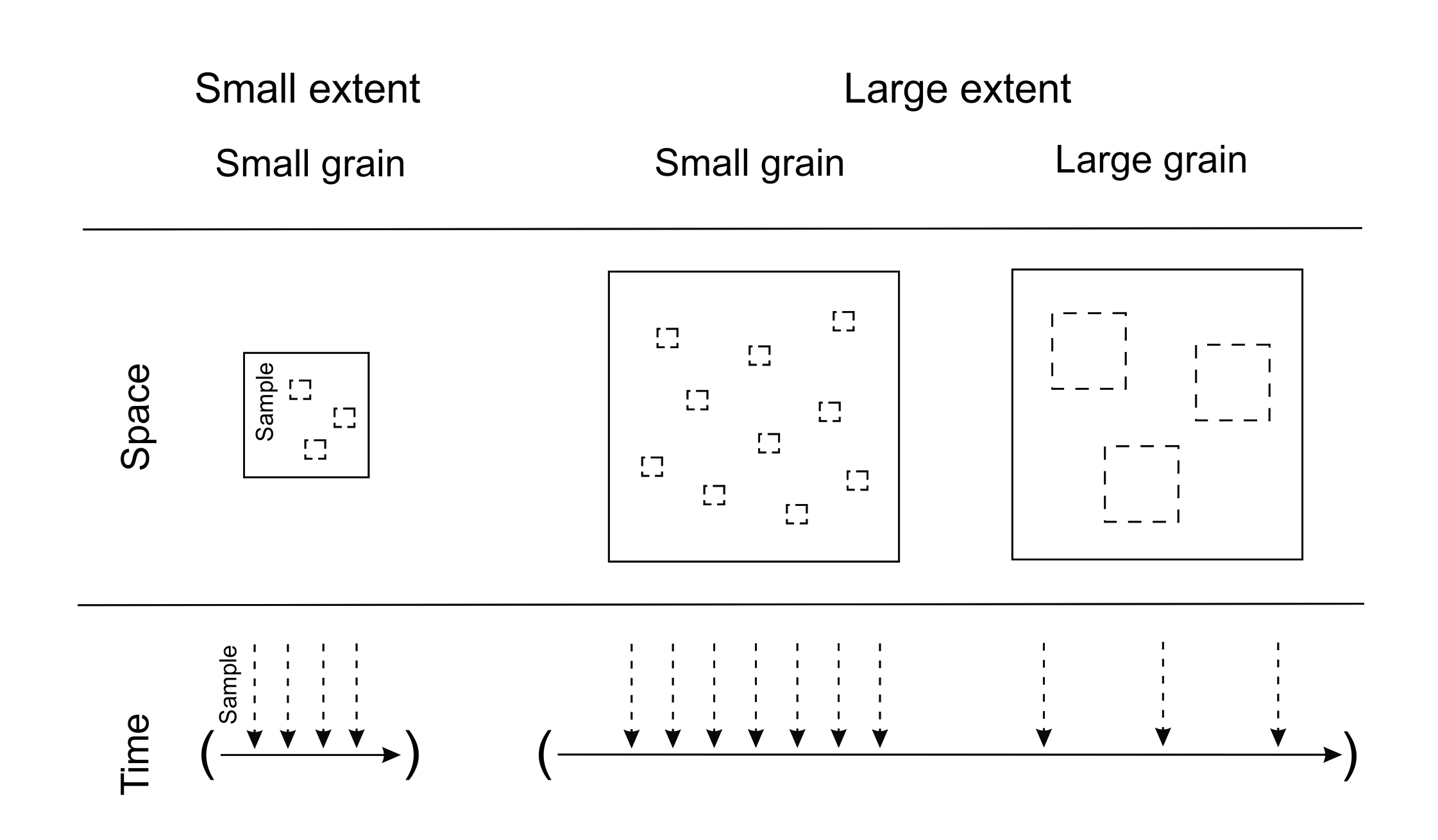
Figure 5.1 Grain and extent. Solid lines represent the total extent of a study in space (squares) or time (arrowed lines in brackets), while dashed lines represent sampling events.

Temporal grain also has additional complexity associated with it, since it can include both frequency and duration (see Ryo et al. 2019 for comprehensive discussion). Over the course of a fortnight-long experiment (extent), temperature might be measured every day (grain). However, these daily temperature readings could be recorded as a spot measurement (i.e. an instantaneous reading), or taken as the average temperature over an hour of recording. The latter incorporates duration, which can also vary, e.g. the duration measured could have been 15 minutes or 2 hours instead. In this chapter, we treat temporal grain in terms of frequency (recurrence interval of spot sampling events, e.g. daily measurements), as this is the more common usage, though we note that duration may also be important. We will return to a discussion of the added complexity of temporal scale relative to spatial scale in a later section. We note that spatial grain may also incorporate density, in terms of the number of sampling units in a given area, which could change geostatistical analysis for example (see Hui et al. 2010). However, we do not consider this further in this chapter.

Because there are two sources of scaling variation (extent and grain), both need to be considered when comparing studies (e.g. in meta-analysis and meta-synthesis). Two studies might be carried out at identical spatial extents and appear to be directly comparable. However, if one was carried out at a smaller grain, it may capture fine-scale environmental heterogeneity or biotic interactions that are not observed in the study with larger grain, even if those factors are equally important in both studies.

We also note that scale is relative for different organisms (Fortin et al. 2021). A study that examines competition at a kilometre scale may appear incomparable to one that examines competition at a metre scale. However, if the studies examine organisms that differ in size (such as lions and ants), the studies may be comparable as those organisms experience competition at their respective study scales (Miguet et al. 2016). The scale at which an organism competes, disperses and so on will vary considerably, and so the appropriate study scale to detect a specific ecological process will also vary (Addicott et al. 1987; Fortin et al. 2012). By the same token, what may appear comparable (e.g. two studies with matching scales) may not be, if the studied taxa differ widely in their spatial and temporal neighbourhoods and ranges.

We will later show how variation in both extent and grain can alter how we interpret patterns, with consequences for synthesising the results of studies executed at different scales.

Box 5.1 Four sources of context dependence

Context dependence occurs when the relationship between two variables varies (or appears to vary) under different conditions. Catford et al. (2022) recently proposed a typology of context dependence, which arises from four sources (Figure 5.2).

The figure shows the relationship between independent variable X and dependent variable Y, with illustrative examples and actions that can reduce unexplained variation and the likelihood of apparent context dependence. ‘Mechanistic context dependence’ (Figure 5.2i) is caused by interaction effects and reflects an underlying ecological process that drives differences between observed relationships. In contrast, ‘apparent context dependence’ (Figure 5.2ii-iv) occurs when the relationship between two variables appears to differ, but in reality does not. A very common type of apparent context dependence is ‘methodological context dependence’ (Figure 5.2iv), where varying methods used by different studies cause observed patterns to differ between them. Scale dependence is a form of apparent context dependence, caused by methodological differences when studies use different grains or extents. Other sources of apparent context dependence include confounding factors and statistical inference.

Confounding factors (Figure 5.2ii) are arguably the hardest to address, because it is likely that multiple factors will affect ecological outcomes, not all of which can be accounted for. Methodological differences are generally easier to address if properly identified, though scale dependence may be an exception (see Can We Retrospectively Correct for Spatial Grain or Extent? in this chapter). Once interacting factors are identified, variation from interaction effects (Fig. 5.2i) should be predictable. The sources of variation are not mutually exclusive and are often interrelated and can manifest in various ways (see Scale Interacts with Other Sources of Context Dependence, this chapter). White boxes show examples only; many other scenarios could occur (for example, different metrics for source in Figure 5.2iv).

 

 

Figure 5.2 Illustration of four sources of context dependence, reprinted from Catford et al. (2022). See text for discussion. ‘Relationship’ is sometimes abbreviated to ‘r’ship’. https://creativecommons.org/licenses/by/4.0//

 

5.2.2 The importance of scale for revealing ecological patterns

The general importance of scale is well understood, and many empirical and theoretical papers have been published on its influence on the observation and interpretation of ecological patterns (e.g. Swenson et al. 2006; Chase et al. 2018; Spake et al. 2021). Scale affects how we view ecological patterns, altering how we see everything from drivers of biodiversity, to the predictors and effects of biological invasions, to the assembly of host-parasite communities (Chase and Knight 2013; Bolnick et al. 2020a). We focus on how this manifests as context dependence (Box 5.1), by impeding the comparison of two or more studies.

Scale is not a property of a system – it is a property of how we observe that system (Fritsch et al. 2020). Indeed, much like ‘populations’ and ‘communities’, it represents a human construct invented to better conceptualise and measure what we observe. An individual plant doesn’t know if we are studying only it, all of the plants of that species in a given field or its global distribution. Scale itself cannot produce or affect ecological processes: it just affects our ability to detect them. In this way, it is important to distinguish spatial and temporal scale from ‘space’ and ‘time’.

Some ecological processes are inherently spatial or temporal: the properties of an ecological system may change through time or in space. This is known as non-stationarity (Rollinson et al. 2021). For example, the relationship between two variables (such as soil nitrogen and plant growth) may vary depending on mean temperature, which varies in space. This is therefore mechanistic context dependence (Box 5.1). The result of non-stationarity is that the mean or variance of ecosystem traits varies through space and time. However, only a certain spatial scale may allow us to detect this (Levin 1992): a study with a small extent might only sample a small temperature range, and the role of soil nitrogen may appear to differ from that of another study with a small extent that sampled a different region of the temperature range. A larger extent would allow for more of the temperature range to be seen (Figure. 5.2iv). We therefore identify ‘scale’ as a source of apparent context dependence (Box 5.1), as it represents a methodological window of observation, rather than an ecological mechanism. While the interaction between spatially or temporally variable ecological processes (non-stationarity) and observational scale poses a problem, it also represents an opportunity.

A careful consideration of scale, particularly if patterns at multiple scales from the same system are compared, can reveal emergent ecological processes (Kopp and Allen 2021). For example, a medium grain may identify the role of the local environmental conditions in determining what species will be present, while a small grain may detect local-scale interspecific competition between those species. When testing a hypothesis, identifying the appropriate spatial and temporal scales of analysis is recommended as the first step in producing suitable models (Miller et al. 2007; Getz et al. 2018). Considering possible scales of analysis encourages us to explicitly consider the link between our observations and the ecological processes driving them. Alternatively, if we want to measure specific mechanisms, thinking about the scale at which we expect to see them will aid in this goal.

We argue that a greater focus on scale dependence therefore provides a dual benefit. First, acknowledging differences in scale between studies will explain some of the apparent context dependence in ecology. Second, scale provides a useful lens to study ecology, as it integrates many processes that determine the distribution and abundance of organisms. Considering multiple scales can inform our understanding and detection of the variation in ecological mechanisms through time and space. While we focus on the former point in this chapter, we highlight the latter where appropriate.

5.2.3 Systems used to explore scale dependence

Through the rest of the chapter, we will use two broad case studies to explore scale dependence. Non-native plants are widely distributed, often representing a large financial cost as well as an ecological threat (Novoa et al. 2021). Their distribution and spread are driven by factors at multiple scales, from global-scale human transport to fine-scale interactions with local native taxa (Smith et al. 2020). Non-native plants provide a useful and highly important system to understand the influence of scale dependence in ecology.

The second case study is host-parasite interactions. Parasites play important roles in ecosystems, from stabilising food webs to influencing the behaviour of individual hosts and the way that whole ecosystems function (Morton et al. 2021; Brian et al. 2022). Parasite community assembly is also strongly hierarchical. A single host can encompass a parasite community: each parasite interacts with the host environment (the environment within the host) as well as other parasites in that environment, including individuals of both the same species and different species (Rynkiewicz et al. 2015). Other factors at larger scales, such as host identity and dispersal limitation, determine the possible pool of parasites that could recruit to a given within-host community (Dallas et al. 2019). Parasite communities, therefore, also provide a convenient system to explore scale dependency in ecology.

5.3 Spatial scale

Both spatial grain and spatial extent could lead to apparent context dependence between studies. In this section, we discuss why this should be so. This leads us to touch upon the importance of considering the traits and life history of organisms when thinking about the appropriate spatial scale of study. We end by showing how it is difficult to correct for spatial scale, and that increased attention needs to be paid to the fact that different ecological processes will be observable at only certain spatial scales.

5.3.1 Spatial grain

The grain of a study can strongly influence its conclusions. This can be seen most clearly in studies that carry out identical analyses at multiple grains.

A recent example comes from Kotowska et al. (2022). The authors explored the relationship between the presence of a plant genus (goldenrods, Solidago spp.) that is non-native in Europe and landscape heterogeneity, which was measured in terms of both diversity (number of different landscape types) and fragmentation. They looked for the presence or absence of goldenrods along replicate transects, and related goldenrod presence to landscape diversity and fragmentation. To investigate the effect of scale, they quantified landscape diversity and fragmentation at different-sized radii around the transect, from 250 to 5000 m (i.e. going from small grain to large grain, Figure 5.1). They found that goldenrod presence was positively associated with both measures of landscape heterogeneity (Kotowska et al. 2022). However, the effect of landscape diversity strengthened with increasing spatial scale, while the effect of fragmentation declined with increasing spatial scale. They surmised that this is likely because landscape diversity generally increases with scale (i.e. a larger grain typically encompasses a greater range of environments), which effectively increases the number and diversity of niches, increasing the likelihood of goldenrods being observed somewhere in that area. In contrast, high fragmentation produces finer-scale disturbance through edge effects, and so strongly facilitates non-native introduction at small scales but less so at larger scales where environmental filtering is more influential than disturbance from edge effects (Kotowska et al. 2022).

The goldenrod example highlights two important points. First, the observed strength of an ecological relationship (between landscape heterogeneity and non-native plant presence) varied depending on the grain examined. Grain is a clear potential source of variation between studies, which could lead to apparent context dependence. If two studies used different grain sizes, they would reach different conclusions about the strength of landscape heterogeneity. Second, this example shows that exploring multiple grain sizes allows assessments to be made about the ecological processes driving non-native plant success. Here, it appears that environmental filtering is an initial, larger-scale driver determining whether goldenrods are present in the general area. Then, their fine-scale position in that area is linked to higher disturbance, which creates spaces for successful establishment.

Spatial grain can also be related to how the organisms in a study are assessed. For example, it may be important to understand how water usage differs between native and non-native plants. One of the most well-known hydrological impacts of plant introductions is the increased water use by non-native plants (Catford 2017). A meta-analysis of over 160 native-introduced species pairs on a range of continents explored the generality of this effect (Cavaleri and Sack 2010). At the leaf scale, evidence suggests that non-native species tend to have greater stomatal conductance than native species, indicating higher water usage (grain size: leaf). However, native and non-native plants were roughly equal in their sap flow rates (grain size: plant), indicating that native and non-native plants had similar water uptake. This difference between the two grain sizes is likely due to a complex combination of leaf properties, canopy cover, and plant age and height. Therefore, the relationship between two variables (plant origin and water use) differs depending on the grain size examined. The example that different patterns are observed between different characteristics of the same organisms also demonstrates that it is difficult to retrospectively correct for scale, as processes can change between scales. It would be incorrect to assume that the effect size seen at the leaf scale could be applied to whole plants.

5.3.2 Spatial extent

The spatial extent of a study may determine how well the study can detect ecological patterns and processes. Two studies conducted at different extents could therefore conclude that different factors are most strongly related to a given response variable, when in reality no such difference exists.

As an example, Bolnick et al. (2020a) explored the factors explaining parasite richness inside freshwater fish (three-spined sticklebacks, Gasterosteus aculeatus) in different lake populations. They included characteristics of the individual fish (e.g. sex, size, gape width) and characteristics of the different lakes (e.g. lake area, elevation, distance from the ocean). Their grain size was the individual fish. However, they carried out their analysis at two different extents: at the within-lake scale (extent: single lake) and the between-lake scale (extent: multiple lakes). They found that some factors, such as host sex, were only important at the single lake extent. Other factors, such as lake area and elevation, were only important at the multiple lake extent. Some factors were also important across both scales, such as host size and gape width. In general, when the extent was a lake, host factors were more important. When the extent was multiple lakes, environmental characteristics become more important (Bolnick et al. 2020a).

These patterns can be interpreted in terms of ecological ‘assembly’. Upon arriving in a new area, organisms need to first be able to survive in the environment and then negotiate biotic interactions in areas of suitable habitat (Götzenberger et al. 2012).

Spatial extent alters our ability to detect these ecological assembly processes. At the extent of single lakes, effects of the broader environmental filters cannot be observed; we are unable to detect that some lakes are more suitable for parasites than others. Instead, parasite patterns appear dominated by biotic factors that occur within a lake, such as host size and how much that host consumes. Only when we make observations at a larger extent can we detect the role of environmental variation in determining why some lakes (and therefore the fish within those lakes) have more parasites than others. Because these processes (environmental filtering, biotic interactions) take place over different spatial scales, our interpretation of what process drives an observed pattern is unavoidably linked with the scale at which we study. Unless two studies take place over identical extents, there is always likely to be some degree of apparent context dependence due to their differential ability to detect the same process.

Host-parasite examples nicely illustrate scale dependence as they help highlight that the same spatial extent can mean different things to different organisms. While the immediate environment for the fish is the lake, the immediate environment for the parasite is the fish, and parasite-parasite competition occurs at the within-fish level. In a paper on the same stickleback-parasite system, within-host parasite-parasite competition was shown to influence parasite abundances (Bolnick et al. 2020b). However, for the fish, interspecific competition occurs within the lake. Therefore, extreme caution is required when comparing studies on organisms that may vary by orders of magnitude in size. An identical spatial extent (e.g. a lake) may give a meaningful signal of competition for a fish, but not for a parasite within that fish. Studies may appear to be context dependent not because a different spatial extent is used, but because the same extent is used to inappropriately compare two organisms whose life history occurs at different scales. These scaling differences between organisms are often underappreciated and can lead to arguments (for example, about the appropriate management of vulnerable populations) (Wiens 1989).

5.3.3 Can we retrospectively correct for spatial grain or extent?

There are techniques for correcting for differences in sampling spatial scales, but it can still be difficult or impossible to eliminate sampling artefacts. We give an example of why this is the case using the relationship between spatial extent and species richness. If two studies are carried out at different extents, researchers may use rarefaction to calculate a standard species richness for a given level of sampling (Chase and Knight 2013). Essentially, this involves moving up or down a species accumulation curve, where the x-axis is spatial extent, and the y-axis is the number of species observed. By estimating the shape of the curve mathematically based on available data it is possible to extrapolate up or down to get an estimate of species richness for a given spatial extent, and standardise that extent across multiple samples or studies.

 

 

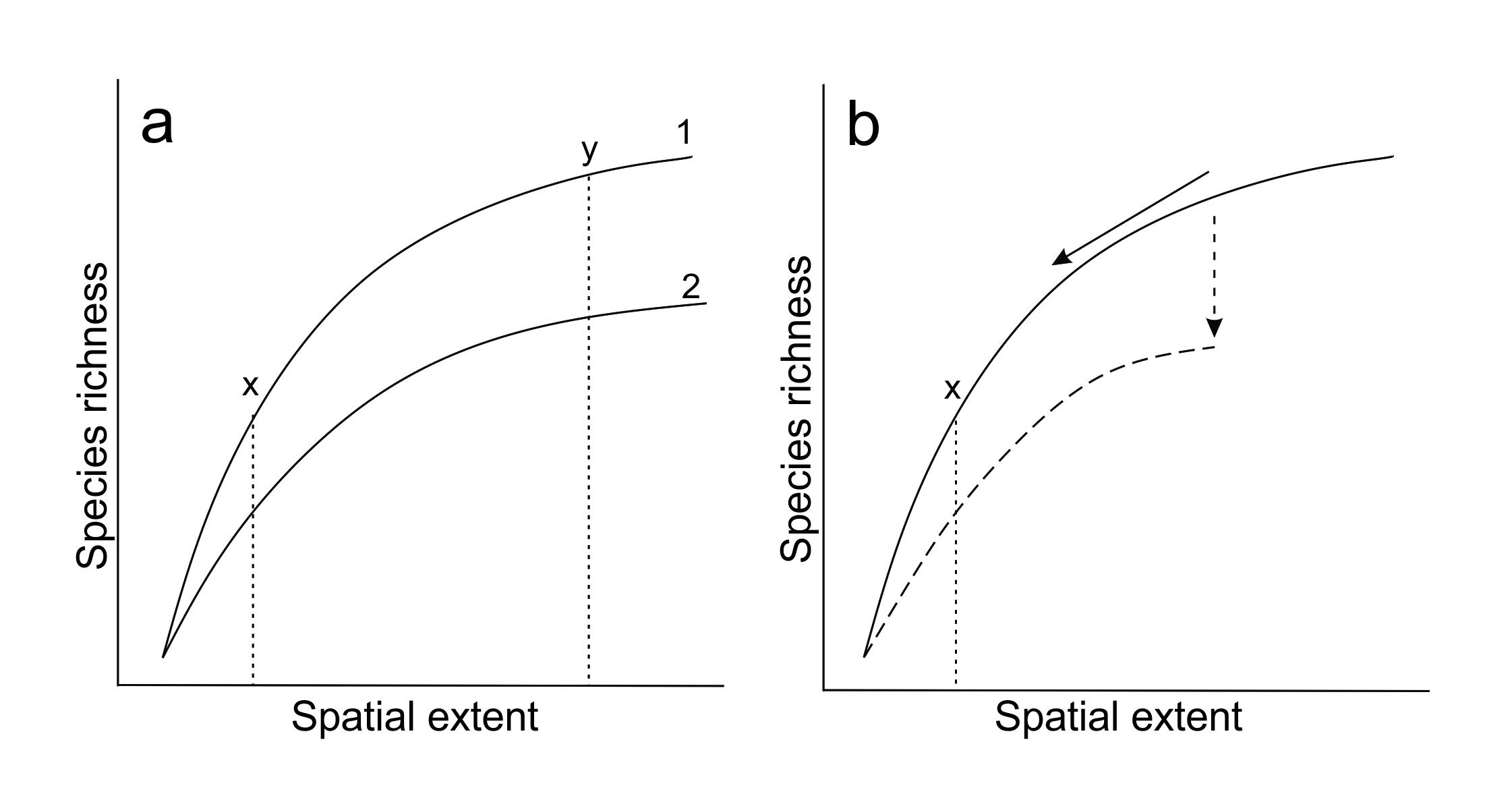
Figure 5.3 Issues when trying to correct for differences in spatial scale. (a) Species accumulation curves from different situations (1 and 2) are unlikely to be parallel, so conclusions still depend on the scale you choose to standardise upon. Adapted from Chase et al. (2018). (b) Ecological processes may change or be lost when spatial extents become smaller (e.g. fragmentation of a previously intact forest), which changes the shape of the species accumulation curve (dashed arrow and line).

There are two problems with the rarefaction approach. The first is that two studies will have different species accumulation curves, that are highly unlikely to be parallel (Figure 5.3a). An attempt to standardise for spatial extent will still be scale dependent because the difference between species accumulation curves varies with what spatial extent is considered (Chase and Knight 2013). The difference between curves 1 and 2 at extent x in Figure 5.3a is only half that at extent y, and the comparison between study 1 and study 2 remains scale dependent.

The second problem is relevant when comparing studies that examine the effect of habitat loss or modification on species responses. Through a disruption of ecological processes (e.g. mutualisms) at smaller scales, species reductions in small and isolated spatial extents are greater than expected (Chase et al. 2020). Therefore, we cannot simply ‘move up and down’ a single species accumulation curve: the entire curve (not just our position on it) will change with the total spatial extent. In Figure 5.3b, the actual species richness when scaling down to extent x will be lower than predicted by the original curve (solid line). To compare between different spatial scales, more sophisticated tools such as Hurlbert’s probability of interspecific encounter are required (see Chase and Knight 2013). Unfortunately, tools such as this are designed specifically for biodiversity comparisons and do not cover all cases of spatial scale dependence.

Another related issue is that of the modifiable areal unit problem (MAUP) (Hui et al. 2010). This problem describes the phenomenon that observed patterns of species distributions will vary with scale, due to spatially explicit processes such as dispersal and social organisation (Peres-Neto and Legendre 2010). Therefore, conclusions about species distributions – for example, the degree of aggregation – remain scale dependent, even if multiple studies are standardised to the same scale. Possible solutions include explicitly including spatial dependence in modelling procedures, though once again this is only suitable for certain types of data (see Dray et al. 2012).

Different spatial grains or extents between studies can cause apparent context dependence. However, the results of any corrections for spatial scale may still not clarify exactly how (and therefore why) two studies differ, because the differences between two studies will vary depending on the scale that is chosen as the ‘standard’ scale for comparison. Because of the tight link between spatial scale and our ability to observe different ecological processes, the best way to deal with spatial context dependence is to carefully consider what processes you are likely to be capturing at your studied extent and the scales over which those processes are likely to occur (Fortin et al. 2012). This will involve considering the scale at which your studied organism lives its life (e.g. how far it can disperse). Comparisons between studies should focus on these qualitative assessments of ecological processes, rather than trying to directly compare between studies at incompatible scales.

5.4 Temporal scale

The temporal context of a study, in terms of both grain and extent, also affects its conclusions. However, there are additional complexities associated with temporal scale relative to spatial scale.

5.4.1 Temporal grain

The frequency at which systems are sampled can affect our conclusions. For example, it is common to model the abiotic niche of species, to predict how species distributions may change with climate change, or to estimate climatically suitable areas that may be vulnerable to non-native introductions. Species distribution models frequently treat environmental variables in terms of their annual average (Karger et al. 2017). However, incorporating environmental variation at smaller grain size, such as quarterly temperature and precipitation extremes, can significantly improve model predictions (Pérez-Navarro et al. 2020).

The chosen temporal grain could alter ecological projections. One species might experience an annual average temperature of 25°C, with an annual range of 20°C–30°C, while another might have an identical average but experience a range of 10°C–40°C. The latter species will likely survive in a much greater range of conditions, and therefore have much stronger potential to spread to other regions. Using a large temporal grain would under-predict this potential (Pérez-Navarro et al. 2020). While incorporating too many variables can lead to poor model performance (see Chapter 7), and gaining good spatial predictions depends on more than choosing a fine temporal scale, considering the variability present in an organism’s life cycle (and our ability to capture it) can improve ecological understanding.

Grain has the capacity to change the resolution at which conclusions can be drawn, and should be considered as a possible explanation for differences between studies that incorporate variables that can vary through time. In this example, refining the grain would provide a better estimate of the true ecological conditions experienced by the organism and facilitate a more accurate assessment of its potential to spread to regions outside its native range. In general, choosing an appropriate grain size is vital to detecting important ecological interactions, such as priority effects which play a major role in early assembly of communities (Fukami 2015).

5.4.2 Temporal extent

The total length or duration of a study can also make the relationship between two variables appear to differ between studies. This is because ecological processes act through time to change observable patterns. For example, there is continued interest in the enemy release hypothesis (ERH) as an explanation for the success of non-native species. The ERH states that non-native species lose their native enemies (parasites, pathogens and predators) when arriving in their new range, and thus experience a competitive advantage over native species (Keane and Crawley 2002). However, enemy loss and gain is a dynamic process. While they may lose their specialist enemies quickly, they can also be targeted by generalists in their new range (Wan et al. 2019). Therefore, non-natives may experience rapid initial release, but then accumulate enemies slowly through time (Hawkes 2007).

If patterns change through time, then studies at different temporal extents have different capacities to detect this (Ryo et al. 2019). In this example, a long-term study would be better placed to detect the fact that enemy pressure is changing – non-native species may begin with much lower enemy richness than natives, but then slowly experience equivalent enemy pressure over time. In contrast, a short-term study would document a ‘snapshot’ of the pattern. The conclusions that the study drew (whether a species was experiencing enemy release or not) would then depend on how soon after initial introduction the study was carried out. If studies are to be fairly compared, there needs to be an acknowledgement that ecological processes change over time and that different temporal extents have different abilities to reflect this.

We recommend, for both temporal extent and grain, that an important first step in dealing with scale dependency comes before a study takes place. The temporal scale of sampling or experimentation should be linked with the process of interest (invasion, enemy release, etc.) and designed to match it. If this is not practical, it should be acknowledged that the study likely captures only a certain part of the process (e.g. likelihood of successful introduction in summer months only; the strength of enemy release ten years after introduction). This will facilitate more informed comparisons between studies.

5.4.3 Do temporal and spatial scale dependence have the same consequences?

So far, we have presented spatial and temporal scale dependence as behaving in a similar fashion. Both are a product of extent and grain, with variation in this extent and grain altering the detection and interpretation of ecological processes. Nonetheless, spatial and temporal scale dependence are not completely analogous. We provide a hypothetical example of this in Figure 5.4 that considers the consequences of changing grain when parasite prevalence varies in both space and time.

 

 

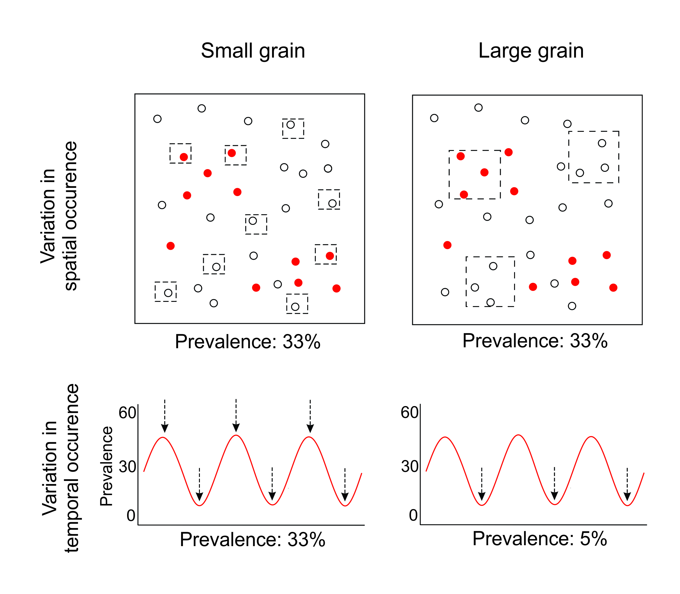
Figure 5.4 Comparing small versus large grains, using a hypothetical example where parasite prevalence is variable in both space and time. Red dots indicate an infected host, while white dots are uninfected hosts.

In space, changing grain may affect our ability to detect the cause of fine-scale parasite distributions (the clusters of red points in Figure 5.4). Small grains would allow parasite distributions to be compared with fine-scale environmental correlates, while larger grains capture broader environmental drivers (Falke and Preston 2022). However, assuming a random distribution of plots in space, small and large spatial grains will recover similar estimated prevalence for a single sampling event (Figure 5.4). This is because larger spatial grains merely average out the variation among smaller spatial grains (Wiens et al. 1989). This is fundamentally different from temporal grain, where larger grains do not average out the pattern observed at smaller grains if parasite prevalence varies throughout the year. Instead, the opposite occurs: they are far more vulnerable to bias due to stochasticity or periodicity (Figure 5.4). Small temporal grains are better able to reliably capture trends. More frequent sampling identifies the periodicity and allows an accurate recording of mean prevalence, while intermittent sampling only ever observes low prevalence.

Both temporal and spatial scale dependence can influence the perceived importance of ecological processes between studies by altering our ability to observe them. Temporal scale dependence is also potentially more likely to produce explicit errors within studies, providing another source of apparent context dependence between studies. This may be because the two aspects of scale (grain and extent) do not apply as neatly to time as they do to space. Spatial grain and extent both cover an area of space: they functionally examine the same metric and can be expressed in the same units. In contrast, while temporal extent covers a period of time, temporal grain technically refers to the frequency of sampling within that period and does not represent a period of time in itself.

Despite this vulnerability, theory concerning temporal scale dependence is less well-developed than that of spatial scale dependence (Ryo et al. 2019). We recommend further attention needs to be paid to the role of temporal grain and extent in producing contradictions between studies. Such work is vital for the assessment of space-for-time substitutions, which have been criticised due to the frequent mismatch between variability in temporal and spatial scales (Damgaard 2019).

5.5 Scale interacts with other sources of context dependence

When comparing between ecological studies, it is unlikely that there will only be one source of variation that could cause context dependence. Instead, both mechanistic context dependence and apparent context dependence could occur simultaneously, and they themselves have diverse sources (Box 5.1).

We now give two extended examples from non-native plant introductions about how spatial and temporal scale interact with each other, and with other sources of context dependence, which can further complicate comparisons between studies.

5.5.1 Darwin’s naturalisation conundrum

Darwin’s ‘naturalisation conundrum’ stems from two opposing predictions made by Darwin (1859). First, he predicted that non-native plants with close phylogenetic relatives in their new range should experience lower growth and fecundity because they will likely have higher trait overlap and therefore compete for similar resources (‘Darwin’s naturalisation hypothesis’, or ‘limiting similarity’). Second, he also predicted that non-native plants with close relatives should be more successful because they will be well-adapted to the environmental conditions there (pre-adaptation hypothesis). Previous work has shown support for both these contrasting hypotheses (e.g. Schaefer et al. 2011; Park and Potter 2013), and the relationship between native and non-native phylogenetic relatedness and non-native success is unclear.

Recent work has suggested that spatial extent (as a source of apparent context dependence) may be responsible for these contradictions. At large extents (regional scale), successful non-native species appear more closely related to native communities than would be expected by chance, because we can detect the role of environmental filtering (Cadotte et al. 2018; Park et al. 2020). Closely related non-natives are more likely to be able to survive the broad environmental conditions in their new range, supporting the pre-adaptation hypotheses. At small extents (local scale), successful non-natives appear less closely related to native communities than would be expected, because they can use different resources to the native species. This minimises competitive exclusion, supporting Darwin’s naturalisation hypothesis. Therefore, non-native species follow a broad pattern of tending to occur in the same region as closely related natives (to match the environment), while spatially segregating over small scales (to avoid competition).

Despite this reasonably intuitive explanation, relying only on spatial extent to reconcile Darwin’s naturalisation conundrum is an over-simplification. Mechanistic context dependence may also have a role to play in determining the relatedness between native and non-native species. For example, at small scales, non-native species tend to be less phylogenetically related to natives in warmer and wetter climates (Park et al. 2020). This pattern may arise because these environments are relatively favourable and homogeneous, and so competition plays a larger role in coexistence. Thus, the context of local environmental conditions also plays a role in the naturalisation conundrum (mechanistic context dependence), but this can only be observed at smaller scales (apparent context dependence).

As another example, phylogenetic relatedness between native and non-native species was strongly dependent on the fire frequency in an oak savanna system, suggesting that both environmental filtering and biotic interactions determine the success of non-native species (Pinto-Ledezma et al. 2020). This pattern also depended on temporal extent. The non-native grass Poa pratensis was generally closely related to species it co-occurred with, supporting the pre-adaptation hypothesis. However, in plots with no fire, this pattern shifted over time until P. pratensis was distantly related to co-occurring species, supporting Darwin’s naturalisation hypothesis (Pinto-Ledezma et al. 2020). Different conclusions would be drawn depending on when the system was studied, or how long it was sampled for. This example shows how the factor of fire frequency (mechanistic context dependence) interacts with temporal extent (which could lead to apparent context dependence) to produce complex ecological patterns, all within a single spatial extent (local scale). These patterns may also present differently across larger spatial scales.

Finally, time since introduction may interact with the ecological effect of non-native species. This could also produce patterns that cause apparent context dependent between studies. In an analysis of plant communities in Auckland, New Zealand, the number of non-native species (i.e. richness) was positively related to the number of native species in the same genus, supporting the pre-adaptation hypothesis. However, the abundance of each of those non-native species was negatively related to native congeners, supporting Darwin’s naturalisation hypothesis and opposing the pre-adaptation hypothesis (Diez et al. 2008). One possible explanation is that non-natives are competitively displacing native species (Cadotte et al. 2018). At early stages of introduction, they appear phylogenetically similar to native species because of environmental filtering. A longer time after introduction, they have competitively displaced closely related native species due to high niche overlap, and so are phylogenetically distant from the remaining native species (Cadotte et al. 2018). Methodological context dependence, in terms of how we choose to measure processes, can influence subsequent interpretation, and requires critical thought.

Various studies show that the observed temporal scale and spatial scale can alter interpretations of interacting factors to produce complex ecological patterns. Considering multiple sources of context dependence simultaneously may be necessary to fairly compare studies that are carried out at different scales and under different ecological conditions. Doing so can help to bring clarity to supposedly contradictory hypotheses, and aid predictions about the circumstances under which certain patterns may be observed.

5.5.2 The invasion paradox

The invasion paradox relates to the relationship between native and exotic species richness. Some studies find that there is a positive relationship between native and non-native species richness, while others find a negative relationship (reviewed in Fridley et al. 2007).

Once again, spatial scale has been implicated as a key cause of this contradiction. Large spatial grains show a positive relationship between native and non-native richness, while small spatial grains show a negative relationship (Peng et al. 2019). This was thought to be for the same reasons as outlined throughout this chapter: at large scales, environmental heterogeneity increases and so more species can be supported, both native and non-native (Fridley et al. 2007). At small scales, competitive interactions are influential and so diverse native communities may resist invasion by using all available resources.

However, multiple additional sources of methodological context dependence may confound the conclusion that spatial grain is responsible for the invasion paradox. Studies with small grains tend to be experiments, which are controlled and explicitly designed to test the effect of native richness on non-native species. In contrast, studies at larger grains and extents are typically observational, which include all the abiotic and biotic variability at a given extent. Therefore, the invasion paradox may be caused by the differences between observational and experimental studies, which are confounded by spatial scale (Peng et al. 2019; Smith and Cote 2019).

Another methodological source of apparent context dependence is the way in which non-native species are assessed. Experiments often use non-native performance (e.g. growth) as a metric of invasive success, while observational studies often use non-native richness (Smith and Cote 2019). These are quite different pieces of information. For example, non-native performance might correlate with non-native abundance and affect native species a lot more than non-native richness. When comparing between studies that use the same metric, the contrast between experimental and observational studies disappears (Smith and Cote 2019).

The invasion paradox shows that there are other methodological sources of apparent context dependence that can covary with spatial scale. Disentangling them, and thus detecting a generalisable ecological signal, requires careful consideration of which ecological processes each method can detect.

5.6 So what?

Different studies will inevitably be carried out at different scales. Two researchers may analyse the same system (or different systems) at different grains, different extents or both, leading to apparent contradictions in their results.

Different sources of scale dependence may interact with each other, or with other forms of context dependence, leading to a complex array of reasons why the conclusions of two studies appear to differ. In order to disentangle true ecological interactions from methodological artefacts, we need to account for the influence of scale, and understand how it influences our interpretation of ecological processes (Spake et al. 2021). Doing so will allow for comparisons between studies that are accurate and informative, and lead to reliable developments in theory and management of ecological systems. Comprehensive guidelines now exist for addressing mechanistic and apparent context dependence as a whole (Box 5.1, Catford et al. 2022). Below, we emphasise the key points that have arisen through this chapter that are specific to scale dependence, which contributes to methodological differences between studies and thus apparent context dependence.

It is becoming increasingly common for a single study to analytically explore different spatial or temporal grains. For a given extent, studies can repeat analyses at different grain sizes (e.g. Dansereau et al. 2022; Kotowska et al. 2022). This can effectively demonstrate how our ability to detect ecological processes changes with scale (Kopp and Allen 2021). We also argue that this approach could make results more comparable between studies, by allowing studies to ‘match’ appropriate grains for comparison. Given that a large majority of studies are restricted to short-term investigations over a small area (Stricker et al. 2015), any approach which expands our knowledge of scale dependence will be of benefit to the wider ecological community.

When studying organisms or environmental factors with known periodicity (e.g. parasite life cycles or climate), we need to acknowledge that one or two samples are unlikely to capture the full story, and try to decrease temporal grain and increase temporal extent where possible (Poulin 2019).

We also need to be aware of how scale relates to statistical inference, another source of context dependence. This is particularly relevant for meta-analyses. Studies with small extents can generally achieve higher replication, and thus receive higher weighting in meta-analyses (Spake et al. 2021). However, they may miss patterns that could be detected at larger scales and bias the meta-analysis conclusions. We have demonstrated that interpretation of ecological processes is heavily scale dependent. Extreme caution is required when synthesising results of multiple studies that may have been carried out over variable scales.

There needs to be an increased emphasis on considering spatial and temporal scale dependence together. Having a fine grain in space does not necessarily mean that all relevant fine-scale processes will be captured if time grain is very coarse.

In general, spatial scale has been considered far more than temporal scale (but see e.g. White et al. 2010). Sophisticated measures exist for accounting for some kinds of spatial scale dependency (Chase and Knight 2013). Methods of accounting for temporal spatial dependence have gained less attention, though work is progressing in this area, particularly in network analysis (e.g. CaraDonna et al. 2021; Fortin et al. 2021) and conservation (e.g. Wauchope et al. 2019). These developments need to be built on to be able to fully account for temporal sampling context.

The scale at which a study is carried out should be informed by the ecological processes expected at that scale. Different questions, such as the role of competition versus the role of temperature in community assembly, can best be answered at different scales, with the former likely requiring a smaller grain than the latter to be effectively observed (Hulme and Bernard-Verdier 2018). This also involves thinking about the traits of the studied organism, such as dispersal. For example, different types of communities (plant, bird, microbial) show different rates of spatial turnover. These differences in turnover are partly explainable by differences in body or propagule size, which covaries with dispersal ability (Graco-Roza et al. 2021). The different scales at which species perceive space and time are vital (Fortin et al. 2021): the same scale may mean different things to different species or functional groups, and cross-study comparisons should take this into account. Because scale affects how we see ecological processes, and processes for different organisms may occur at different scales, we cannot merely standardise for scale (Chase et al. 2019). We need to think critically about the relationship between processes, organisms and scale.

Finally, it may be that studies at different scales cannot be effectively compared. If this is the case, synthesis should be attempted cautiously, with comparisons being very explicit when it comes to scale. Attempting to develop ecological theory by comparing studies that answer different questions – by virtue of being carried out at different scales – may be misleading and will exacerbate rather than ameliorate confusion about ecological patterns and the processes driving them.

As a discipline, Ecology will ideally move from declaring a result as ‘context dependent’ to exploring and explaining why conclusions appear different between studies. Accounting for study scale, and its interaction with other sources of context dependence, is one important way of reconciling apparently contradictory or variable results. Doing so will allow us to better understand how methodological choices and inference strategies can affect ecological interpretations. Ultimately, understanding and accounting for these sources of bias will lead to greater mechanistic understanding of the factors and processes that drive variation in ecology.

5.7 References

Addicott, J. F., J. M. Aho, M. F. Antolin, et al. 1987. Ecological neighborhoods: scaling environmental patterns. Oikos 49:340-346.

Bolnick, D. I., E. J. Resetarits, K Ballare, Y. E. Stuart, and W. E. Stutz. 2020a. Host patch traits have scale‐dependent effects on diversity in a stickleback parasite metacommunity. Ecography 43:990-1002. doi:10.1111/ecog.04994

Bolnick, D. I., E. J. Resetarits, K. Ballare, Y. E. Stuart, and W. E. Stutz. 2020b. Scale‐ dependent effects of host patch traits on species composition in a stickleback parasite metacommunity. Ecology 101:e03181. doi:10.1002/ecy.3181

Brian, J. I., S. A. Reynolds, and D. C. Aldridge 2022. Parasitism dramatically alters the ecosystem services provided by freshwater mussels. Functional Ecology 36:2019-2042. doi:10.1111/1365-2435.14092

Cadotte, M. W., S. E. Campbell, S. P. Li, D. S. Sodhi, and N. E. Mandrak. 2018. Preadaptation and naturalization of nonnative species: Darwin’s two fundamental insights into species invasion. Annual Review of Plant Biology 69:661-684. doi:10.1146/annurev-arplant-042817-040339

Carlile, D. P. N., F. Zino, C. Natividad, and D. B. Wingate 2003. A review of four successful recovery programmes for threatened sub-tropical petrels. Marine Ornithology 31:185-192.

Catford, J. A. 2017. Hydrological impacts of biological invasions. In Impact of biological invasions on ecosystem services, eds M. Vilà and P. E. Hulme, 63-80. Cham: Springer. doi:10.1007/978-3-319-45121-3_5

Catford, J. A., J. R. Wilson, P. Pyšek, P., P. E. Hulme, and R. P. Duncan. 2022. Addressing context dependence in ecology. Trends in Ecology and Evolution 37:158-170. doi:10.1016/j.tree.2021.09.007

Cavaleri, M. A., L. and Sack. 2010. Comparative water use of native and invasive plants at multiple scales: a global meta‐analysis. Ecology 91:2705-2715. doi:10.1890/09-0582.1

Chase, J. M., and T. M. Knight. 2013. Scale‐dependent effect sizes of ecological drivers on biodiversity: why standardised sampling is not enough. Ecology Letters 16:17-26. doi:10.1111/ele.12112

Chase, J. M., B. J. McGill, D. J. McGlinn, et al. 2018. Embracing scale‐dependence to achieve a deeper understanding of biodiversity and its change across communities. Ecology Letters 21:1737-1751. doi:10.1111/ele.13151

Chase, J. M., B. J. McGill, P. L. Thompson, et al. 2019. Species richness change across spatial scales. Oikos 128:1079-1091. doi:10.1111/ele.13151

Chase, J. M., S. A. Blowes, T. M. Knight, K. Gerstner, and F. May. 2020. Ecosystem decay exacerbates biodiversity loss with habitat loss. Nature 584:238-243. doi:10.1038/s41586-020-2531-2

Connolly, S. R., M. A. MacNeil, M. J. Caley, et al. 2014. Commonness and rarity in the marine biosphere. Proceedings of the National Academy of Sciences of the United States of America 111:8524-8529. doi:10.1073/pnas.1406664111

Crawley, M. J., and J. E. Harral. 2001. Scale dependence in plant biodiversity. Science 291:864-868. doi:10.1126/science.291.5505.864

Dallas, T. A., A. L. Laine, and O. Ovaskainen. 2019. Detecting parasite associations within multi-species host and parasite communities. Proceedings of the Royal Society B: Biological Sciences 286:20191109. doi:10.1098/rspb.2019.1109

Damgaard, C. 2019. A critique of the space-for-time substitution practice in community ecology. Trends in Ecology and Evolution 34:416-421. doi:10.1016/j.tree.2019.01.013

Dansereau, G., P. Legendre, and T. Poisot. 2022. Evaluating ecological uniqueness over broad spatial extents using species distribution modelling. Oikos 2022:e09063. doi:10.1111/oik.09063

Darwin, C. 1859. On the origin of species by means of natural selection, or the preservation of favoured races in the struggle for life. London: John Murray.

Diez, J. M., J. J. Sullivan, P. E. Hulme, G. Edwards, and R. P. Duncan. 2008. Darwin’s naturalization conundrum: dissecting taxonomic patterns of species invasions. Ecology Letters 11:674-681. doi:10.1111/j.1461-0248.2008.01178.x

Dray, S., R. Pélissier, P. Couteron, et al. 2012. Community ecology in the age of multivariate multiscale spatial analysis. Ecological Monographs 82:257-275. doi:10.1890/11-1183.1

Falke, L. P., and D. L. Preston. 2022. Freshwater disease hotspots: Drivers of fine‐scale spatial heterogeneity in trematode parasitism in streams. Freshwater Biology 67:487-497. doi:10.1111/fwb.13856

Fortin, M. J., P. M. James, A. MacKenzie, et al. 2012. Spatial statistics, spatial regression, and graph theory in ecology. Spatial Statistics 1:100-109. doi:10.1016/j.spasta.2012.02.004

Fortin, M. J., M. R. T. Dale, and C. Brimacombe. 2021. Network ecology in dynamic landscapes. Proceedings of the Royal Society B 288:20201889. doi:10.1098/rspb.2020.1889

Frankish, C. K., R. A. Phillips, T. A. Clay, M. Somveille, and A. Manica. 2020. Environmental drivers of movement in a threatened seabird: insights from a mechanistic model and implications for conservation. Diversity and Distributions 26:1315-1329. doi:10.1111/ddi.13130

Fridley, J. D., J. J. Stachowicz, S. Naeem, et al. 2007. The invasion paradox: reconciling pattern and process in species invasions. Ecology 88:3-17. doi:10.1890/0012-9658(2007)88[3:TIPRPA]2.0.CO;2

Fritsch, M., H. Lischke, and K. M. Meyer. 2020. Scaling methods in ecological modelling. Methods in Ecology and Evolution 11:1368-1378. doi:10.1111/2041-210X.13466

Fukami, T. 2015. Historical contingency in community assembly: integrating niches, species pools, and priority effects. Annual Review of Ecology, Evolution, and Systematics 46:1-23. doi:10.1146/annurev-ecolsys-110411-160340

Getz, W. M., C. R. Marshall, C. J. Carlson, et al. 2018. Making ecological models adequate. Ecology Letters 21:153-166. doi:10.1111/ele.12893

Götzenberger, L., F. de Bello, K. A. Bråthen, et al. 2012. Ecological assembly rules in plant communities: Approaches, patterns and prospects. Biological Reviews 87:111-127. doi:10.1111/j.1469-185X.2011.00187.x

Graco‐Roza, C., S. Aarnio, N. Abrego, et al. 2022. Distance decay 2.0 – a global synthesis of taxonomic and functional turnover in ecological communities. Global Ecology and Biogeography 31:1399-1421. doi:10.1111/geb.13513

Hawkes, C. V. 2007. Are invaders moving targets? The generality and persistence of advantages in size, reproduction, and enemy release in invasive plant species with time since introduction. The American Naturalist 170:832-843. doi:10.1086/522842

Hui, C., R. Veldtman, and M. A. McGeoch. 2010. Measures, perceptions and scaling patterns of aggregated species distributions. Ecography 33:95-102. doi:10.1111/j.1600-0587.2009.05997.x

Hulme, P. E., and M. Bernard‐Verdier. 2018. Comparing traits of native and alien plants: Can we do better? Functional Ecology 32:117-125. doi:10.1111/1365-2435.12982

Karger, D. N., O. Conrad, J. Böhner, et al. 2017. Climatologies at high resolution for the earth’s land surface areas. Scientific Data 4:1-20. doi:10.1038/sdata.2017.122

Keane, R. M., and M. J. Crawley. 2002. Exotic plant invasions and the enemy release hypothesis. Trends in Ecology and Evolution 17:164-170. doi:10.1016/S0169-5347(02)02499-0

Kopp, D., and D. Allen. 2021. Scaling spatial pattern in river networks: The effects of spatial extent, grain size and thematic resolution. Landscape Ecology 36:2781-2794. doi:10.1007/s10980-021-01270-2

Kotowska, D., T. Pärt, P. Skórka, et al. 2022. Scale dependence of landscape heterogeneity effects on plant invasions. Journal of Applied Ecology 59:1313-1323. doi:10.1111/1365-2664.14143

Lawton, J. H. 1999. Are there general laws in ecology? Oikos 84:177-192.

Levin, S. A. 1992. The problem of pattern and scale in ecology: The Robert H. MacArthur award lecture. Ecology 73:1943-1967.

Miguet, P., H. B. Jackson, N. D. Jackson, et al. 2016. What determines the spatial extent of landscape effects on species? Landscape Ecology 31:1177-1194. doi:10.1007/s10980-015-0314-1

Miller, J., J. Franklin, and R. Aspinall. 2007. Incorporating spatial dependence in predictive vegetation models. Ecological Modelling 202:225-242. doi:10.1016/j.ecolmodel.2006.12.012

Mitchell, E. G., S. Harris, C. G. Kenchington, et al. 2019. The importance of neutral over niche processes in structuring Ediacaran early animal communities. Ecology Letters 22:2028-2038. doi:10.1111/ele.13383

Morton, D. N., C. Y. Antonino, F. J. Broughton, et al. 2021. A food web including parasites for kelp forests of the Santa Barbara Channel, California. Scientific Data 8:1-14. doi:10.1038/s41597-021-00880-4

Münkemüller, T., L. Gallien, L. J. Pollock, et al. 2020. Dos and don’ts when inferring assembly rules from diversity patterns. Global Ecology and Biogeography 29:1212-1229. doi:10.1111/geb.13098

Novoa, A., D. Moodley, J. A. Catford, et al. 2021. Global costs of plant invasions must not be underestimated. NeoBiota 69:75-78. doi:10.3897/neobiota.69.74121

Park, D. S., and D. Potter. 2013. A test of Darwin’s naturalization hypothesis in the thistle tribe shows that close relatives make bad neighbors. Proceedings of the National Academy of Sciences of the United States of America 110:17915-17920. doi:10.1073/pnas.1309948110

Park, D. S., X. Feng, B. S. Maitner, et al. 2020. Darwin’s naturalization conundrum can be explained by spatial scale. Proceedings of the National Academy of Sciences of the United States of America 117:10904-10910. doi:10.1073/pnas.1918100117

Peres‐Neto, P. R., and P. Legendre. 2010. Estimating and controlling for spatial structure in the study of ecological communities. Global Ecology and Biogeography 19:174-184. doi:10.1111/j.1466-8238.2009.00506.x

Poulin, R. 2019. Best practice guidelines for studies of parasite community ecology. Journal of Helminthology 93:8-11. doi:10.1017/S0022149X18000767

Peng, S., N. L. Kinlock, J. Gurevitch, and S. Peng. 2019. Correlation of native and exotic species richness: a global meta‐analysis finds no invasion paradox across scales. Ecology 100:e02552. doi:10.1002/ecy.2552

Pérez‐Navarro, M. A., O. Broennimann, M. A. Esteve, et al. 2021. Temporal variability is key to modelling the climatic niche. Diversity and Distributions 27:473-484. doi:10.1111/ddi.13207

Pinto‐Ledezma, J. N., F. Villalobos, P. B. Reich, J. A. Catford, D. J. Larkin, and J. Cavender‐Bares. 2020. Testing Darwin’s naturalization conundrum based on taxonomic, phylogenetic, and functional dimensions of vascular plants. Ecological Monographs 90:e01420. doi:10.1002/ecm.1420

Rollinson, C. R., A. O. Finley, M. R. Alexander, et al. 2021. Working across space and time: nonstationarity in ecological research and application. Frontiers in Ecology and the Environment 19:66-72. doi:10.1002/fee.2298

Rynkiewicz, E. C., A. B. Pedersen, and A. Fenton. 2015. An ecosystem approach to understanding and managing within-host parasite community dynamics. Trends in Parasitology 31:212-221. doi:10.1016/j.pt.2015.02.005

Ryo, M., C. A. Aguilar-Trigueros, L. Pinek, et al. 2019. Basic principles of temporal dynamics. Trends in Ecology and Evolution 34:723-733. doi:10.1016/j.tree.2019.03.007

Sandel, B., and A. B. Smith. 2009. Scale as a lurking factor: incorporating scale‐dependence in experimental ecology. Oikos 118:1284-1291. doi:10.1111/j.1600-0706.2009.17421.x

Schaefer, H., O. J. Hardy, L. Silva, et al. 2011. Testing Darwin’s naturalization hypothesis in the Azores. Ecology Letters 14:389-396. doi:10.1111/j.1461-0248.2011.01600.x

Smith, N. S., and I. M. Cote. 2019. Multiple drivers of contrasting diversity–invasibility relationships at fine spatial grains. Ecology 100:e02573. doi:10.1002/ecy.2573

Spake, R., A. S. Mori, M. Beckmann, et al. 2021. Implications of scale dependence for cross‐study syntheses of biodiversity differences. Ecology Letters 24:374-390. doi:10.1111/ele.13641

Stricker, K. B., D. Hagan, and S. L. Flory. 2015. Improving methods to evaluate the impacts of plant invasions: Lessons from 40 years of research. AoB Plants 7:plv028. doi:10.1093/aobpla/plv028

Swenson, N. G., B. J. Enquist, J. Pither, et al. 2006. The problem and promise of scale dependency in community phylogenetics. Ecology 87:2418-2424. doi:10.1890/0012-9658(2006)87[2418:TPAPOS]2.0.CO;2

Turner, M. G., V. H. Dale, and R. H. Gardner. 1989. Predicting across scales: theory development and testing. Landscape Ecology 3:245-252.

Wan, J., B. Huang, H. Yu, and S. Peng. 2019. Reassociation of an invasive plant with its specialist herbivore provides a test of the shifting defence hypothesis. Journal of Ecology 107:361-371. doi:10.1111/1365-2745.13019

Wauchope, H. S., T. Amano, W. J. Sutherland, and A. Johnston. 2019. When can we trust population trends? A method for quantifying the effects of sampling interval and duration. Methods in Ecology and Evolution 10:2067-2078. doi:10.1111/2041-210X.13302

Wiens, J. A. 1989. Spatial scaling in ecology. Functional Ecology 3:385-397.