7 Assumptions: Respecting the known unknowns

Bruce Webber , Roger Cousens and Daniel Atwater

How to cite this chapter

Webber B. L., Cousens R. D. and Atwater D. Z. (2023) Assumptions: respecting the known unknowns. In: Cousens R. D. (ed.) Effective ecology: seeking success in a hard science. CRC Press, Taylor & Francis, Milton Park, United Kingdom, pp. 97-126. Doi:10.1201/9781003314332-7

Abstract Assumptions are ubiquitous in science. We use them to simplify nature so that we can understand it intellectually, and to permit progress despite knowledge gaps, thus allowing for the development and application of ecological understanding. If our assumptions are at least approximately valid, then we can draw valuable insights and cast reliable projections. If not, assumptions can cause us and our stakeholders to be confused or seriously misled. In this chapter we pull apart research in one topical area – niche theory and its applicability to the modelling of species distributions – to illustrate just how many assumptions we make and how important they are. Our focus involves the question of whether species alter their niches when they spread into a new region, what such a conclusion would mean ecologically and how widely species can spread as a result. Assumptions are made in the formulation of the concept of the niche, in the properties of the data that are analysed, in the construction of the models that are used in the analyses and in the inferences that we ultimately draw. Yet, it is common for researchers to be unaware of even the most basic of these assumptions. All ecological researchers need to familiarise themselves with the assumptions implicit and explicit in their methods, to appreciate the consequences of their findings, the subsequent applications if those assumptions turn out to be inappropriate and to communicate those limitations to readers. Every opportunity should be taken to rigorously check the validity of assumptions using whatever means are available. Without such routine evaluation, every reader of our work would be justified in doubting our conclusions.

7.1 The biggest ‘elephant in the room’?

Ecology is built on and enabled by assumptions.

Just about everything we do, from measuring the length of a leaf or the pH of a liquid to the most complex of bioinformatic analyses or mathematical models, requires assumptions. An assumption is something that is believed to be true, or considered to be true for the sake of argument, but is not known to be true.

By making assumptions, we can simplify nature so that we can deal with it intellectually and effectively. For example, we can assume that there are things that we call populations, communities and ecosystems, even though these are human constructs. We assume that these entities have traits with which we decide to imbue them, such as size, diversity, resilience and energy flow. We assume that we can devise qualities and quantities that adequately represent those traits. We assume that the data that we then collect are appropriate, accurate and unbiased. We assume that our models are adequate representations of reality (Wiens et al. 2009) and that the assumptions of the statistical methods that we use are robust. And we make assumptions every time we draw inferences from our results, such as whether, how and why the results are statistically, biologically, economically or socially of any relevance. Indeed, the entire research process, from its conception to its final conclusions, consists of layers and combinations of assumptions (Schröter et al. 2021). Our science, therefore, is no better than the assumptions that we make.

Every time we make an assumption, we run the risk of making a mistake: every assumption has the potential to be false. This reality may not matter in many instances, as long as the assumption is close enough to the truth. Some methods that we use may be relatively insensitive to a particular assumption, especially if the error is the same across all of the entities that we are comparing. If we overlook the assumption that a ruler – and where we choose to place it – gives accurate measurement of length, the consequences may be minor, especially if the same person always makes the measurements. Likewise, the assumption that we can accurately measure vegetation cover with a visual assessment of a quadrat is often a known source of bias. Yet again, as long as we do not make comparisons of cover across studies by different people, or if the effect size we detect is large, then the bias may be inconsequential.

But some things we do can be highly sensitive to erroneous assumptions. For example, failure to correct for departure from homogeneity of variance can be sufficient to convert an interpretation of a statistically ‘significant’ result to one of ‘non-significant’ (Cousens 1988). If we fail to recognise an important assumption, check its validity or consider the consequences if it is wrong, then potentially we can mislead ourselves as well as those engaging with our work. If assumptions are our windows on the world, then we need to make sure we scrub them off every once in a while to ensure that the light still comes in (Alda 1980 in Ratcliffe 2017).

Many assumptions in ecology are implicit and we do not bother to explore them every time we make them. When we say that we are studying ‘population dynamics’ we seldom define ‘population’ unambiguously. We may not specify how we attribute individuals to a particular population, where the boundaries of the population are or even whether we are assuming random mating and homogeneity within the population. We either take it for granted that the reader will fully appreciate the assumptions that we are making, or that any failure to appreciate them is of little consequence.

Other times, we state our assumptions explicitly because we, and our peers, know that they matter, or because there is a culture of defining certain assumptions. Sometimes we comment on specific analyses that we have conducted in order to show that we have checked that the assumptions are at least approximately correct.

There is a great deal of variation among researchers in their familiarity with the importance of particular assumptions – and in whether or not the scientist explores the validity of these assumptions. A failure to address critical assumptions is likely to occur when someone picks up an unfamiliar machine or a piece of common user-friendly software and applies it without being adequately trained. It takes time and experience to acquire skills in applying the methods, to become aware of the existence of key assumptions and to appreciate the need (and find time) to adequately address them. Casual users of ecological methods may never develop a high level of skill in their application. Until assumptions are given greater consideration in the design of research, their limitations better acknowledged during data interpretation and suitable caveats stated explicitly in discussions of results, scientific progress can be compromised.

As we will show, published ecological research contains a high frequency of errors, even in situations where it would be quite straightforward to avoid them. Moreover, the reasons for this threat to best practice ecological standards are often complex and frequently not attributable to ignorance alone.

If our research is only as good as the assumptions that we make, then the onus is on every scientist to make themselves aware of their assumptions – preferably before they carry out the research (so that they can minimise the effect on the data) and definitely after they have collected the data (so that they can take post hoc action and select appropriate language to minimise the probability of a false inference). Equally, end-users of our research need to be aware of the assumptions commonly made by scientists, and the pitfalls that can be encountered when applying that research to particular problems.

While readers of our publications should be able to expect that we have considered all relevant assumptions, the research publication and peer review system is an imperfect quality control system. For reasons of tradition or concern for space, it is not standard practice for every publication to list every assumption that is made. Indeed, we should be able to expect adherence to many basic procedures that ought to be known (so-called ‘best practice’). Some scientists would even consider it demeaning to be asked to demonstrate that basic procedures have been followed (such as where we place a ruler against the stem to measure seedling height). But the fact of the matter is that not every author of an article and not every reader actually knows what all the assumptions made in the research are, which ones are important or how they ought to have been checked. A collective effort is required to ensure that ecological assumptions are ‘safe’ for a given context.

In this chapter, we present the detection of niche shifts for introduced plants as a case study for exploring ecology’s reliance on assumptions. We have chosen this example because it is timely, because it illustrates the powers and pitfalls of assumptions in ecological research and because we as authors have long nurtured our own frustrations with the standards tolerated of research in this area and the role of assumptions both spoken and unspoken.

This chapter is very long, but necessarily so, because we seek to illustrate just how many assumptions can be hidden within a few lines of text in a concise scientific article. Unlike the other chapters that consider the breadth of ecology or superficially cover entire fields of research, this chapter is a detailed critique of a single research topic in its entirety. The reader is challenged to stay with us through the lengthy discourse, even if niche shifts are not their area of interest. They will hopefully learn how to undertake such a detailed forensic analysis of their own research projects: it can be both eye-opening and jaw-dropping!

To make any scientific headway on species’ niches requires two basic assumptions and a number of subsequent ones. Firstly, we must assume that the thing we choose to call the ‘niche’ serves a useful scientific purpose. Secondly, that we can measure it. Both of these assumptions are widely taken for granted, but they deserve closer scrutiny. We can only measure the niche by making a series of further assumptions in relation to the data that we use and the analyses that we perform. To make the next step, to draw conclusions from the results, requires yet further assumptions. These assumptions conspire to create a morass of cascading uncertainty that if ignored threatens to derail any hope of progress. But if fully appreciated and carefully managed, assumptions are the great enablers of progress in ecology.

7.2 The species’ niche concept

Ecology is awash in words and concepts that instantly mean something to most people, but not necessarily the same thing to all people. Many of them – the niche is a good example – were adopted from other non-scientific uses and at a time in ecology’s early history when we were still grappling with basic concepts.

Early definitions of the niche were vague, because ecological paradigms were still being defined. Each species was regarded as having a way that it fitted within the communities and ecosystems in which it was found. This was termed the ‘niche’ of a species, referring both to the role that species played in an ecosystem and to the species’ general ecological needs.

This early conceptualisation of the niche was a species-level attribute, assuming that any infraspecific variation was of little consequence. For non-specialists, it is sufficient to define the niche as the role a species plays in an ecosystem. Yet, as specialists searched for ever-greater levels of ecological understanding, it was inevitable that they found a need for language that was semantically more precise and less conceptually ambiguous, allowing us to communicate subtleties of meaning and to become more quantitative.

There are two distinct ways in which ecologists have come to view the niche of a species. To those involved in the development of theory relating to community structure, the niche concerns the way in which a species accesses the resources it needs to survive and reproduce. It is about how different species impact on one another within a given location, how local processes may have caused these patterns of resource use to evolve, what governs species’ coexistence, and thus community diversity. This functional role of a species is often referred to as the Eltonian niche, after Charles Elton who pioneered such thinking. Elton developed this concept in turn after Grinnell’s (1917) first definition of the niche, as a layer in a hierarchy of forces that controlled the distribution and abundance of species. In the same seminal paper, Grinnell advanced the competitive exclusion principle. This role-centred view of the niche has, since its inception, been entangled with species’ coexistence.

The other commonly considered concept of the niche, which will concern us from here onwards, is usually referred to as the Hutchinsonian niche, after G. Evelyn Hutchinson. This niche concept relates to the tolerance limits of an individual species to the various biotic and abiotic components of its environment. Hutchinson (1978) distinguished between ‘scenopoetic’ environmental variables, the extrinsic and immutable conditions an organism experiences in the course of its life (Begon et al. 1996), such as temperature, humidity, concentrations of gases and pH, and ‘bionomic’ variables, the labile resources that organisms must access, such as light, nutrients and water. Hutchinson defined the ‘fundamental species niche’ as the n-dimensional environmental hypervolume, based on these variables, containing all possible environments within which the species could persist indefinitely. If we are able to validly measure responses to these variables, we can make interesting comparisons between the environmental preferences of the species (as Hutchinson and many others have since done).

Hutchinson pointed out that the niches of species are not independent of one another. If a part of the scenopoetic environment is occupied by a competitor, fewer resources will be available because of competition. In other words, the bionomic variables will be reduced, potentially resulting in a net reproductive rate \(\lambda\) < 1 and excluding the species from those environments. Predation and herbivory will have similar effects, reducing (or precluding) the species’ ability to capture bionomic resources. We might also extend this thinking to mutualist species such as a pollinator, which might constitute bionomic resources in their own right. Hutchinson therefore introduced the term ‘realised niche’ for the region of the fundamental niche that the species can occupy in the presence of other species.

The assumption of a species having a fixed environmental tolerance range – a niche – is, of course, naïve. We should not forget either that the very concept of a species is an assumption in and of itself, which often does not stand up to more detailed interrogation. The principle of natural selection is based on the assumption that individuals vary in their environmental tolerances. The match between the individual’s tolerance curve and its environment determines how many of their progeny will be available for the next generation. As a result, populations in different environments could evolve different tolerance limits. Indeed, if we were to ignore convention, we might refer to all levels of this hierarchical series of tolerance ranges, of individuals, populations, subspecies and species as niches.

From an evolutionary point of view, then, we can develop a population genetics definition of the Hutchinsonian fundamental species niche – though still an abstract and naïve one. If sufficient numbers and genotypes of the species were to arrive (i.e. enough for establishment) into every possible environment from every suitable occupied environment, and they reproduce, mutate and adapt indefinitely with limited subsequent dispersal, then the fundamental niche of the species would be all those environments in which populations would have a finite population growth rate \(\lambda\) ≥ 1. However, the more we think about the detail of this model of the fundamental niche, the more we expose creakiness in the concept. Even the optimal distribution of a species depends upon its particular ecology. The population dynamics of such a system will depend upon emigration and immigration among subpopulations, and not all subpopulations will be perfectly adapted to the regions they inhabit, particularly at range edges. Further, evolution to biological aspects of the niche, such as competition and predation, may trade-off against abiotic conditions, such as temperature and soil conditions.

7.3 The niche concept meets the real world

If we believe that the fundamental niche of a species is something that is worth knowing, can we measure it? Quite simply, the answer is ‘no’. It is impossible to quantify experimentally the n-dimensional hypervolume that constitutes a niche: there are simply too many possible combinations for us to recreate effectively. Even if we know a priori which subset of environmental variables is the most important, it is difficult to design experimental protocols in which to measure their tolerances, particularly for interactions between variables. Many complexities are difficult to resolve, such as the creation of sufficiently natural conditions, keeping long-lived species healthy and behaving naturally, the calculation of \(\lambda\) (and not a component of it or some surrogate measure) and which genotypes to work with (as we discussed earlier, not all genotypes will have the same tolerances). The fundamental niche is an entirely theoretical concept.

We can measure something about a species’ niche, and this has become popular among ecologists, but it is definitely not the fundamental niche. Most commonly, we do this by resorting to the incomplete and biased information provided by the geographic distribution of species. The fundamental niche of the species determines the set of locations on the globe where the species could potentially persist. So, the distribution of a species must tell us something about the niche. If we comprehensively map a species and then measure all the relevant environmental variables at every location, we could – in some way – depict the suite of environments actually occupied. The jargon in this area of work is that we collect data in geographic space (G-space) and convert it to data in environmental space (E-space).

The problem is that species’ geographic distributions past and present represent only a (biased) subset of potentially suitable environments. There are three main reasons for this. Firstly, the vagaries of our planet – the positions of our oceans and land masses, the types and locations of climates and soils, and so on – mean that only a subset of environments within the fundamental niche actually exist for the species ever to experience (referred to as the potential niche by Jackson and Overpeck 2000). Secondly, other organisms will be present and their interactions may prevent the species from persisting in scenopoetic environments that would otherwise be suitable. The region in which the species does persist, despite these biotic interactions, is Hutchinson’s realised niche sensu lato. Thirdly, the species may be absent from regions of suitable E-space because it has never been able to reach them or, if it has, it has been unable to establish for some reason. We will refer to the occupied E-space that results from all three circumstances as the realised niche sensu stricto.

We present a two-dimensional representation of this in Figure 7.1. The ranges of two scenopoetic variables within which a population can potentially persist (\(\lambda\) ≥ 1) is the fundamental niche (blue ellipse). Reductions in availability of resources, interactions with further scenopoetic variables and with other species combine to reduce the extents of the variables for which \(\lambda\) ≥ 1 (red ellipse). In addition, only some combinations of suitable variables (green shaded areas) actually exist within the region of study. The species will therefore only occur (black dots) in the environments for which the green areas and the red ellipse overlap – provided that it has been able to reach and establish there (the hatched area is unoccupied due to dispersal limitation). We refer to this as the realised niche sensu stricto.

 

 

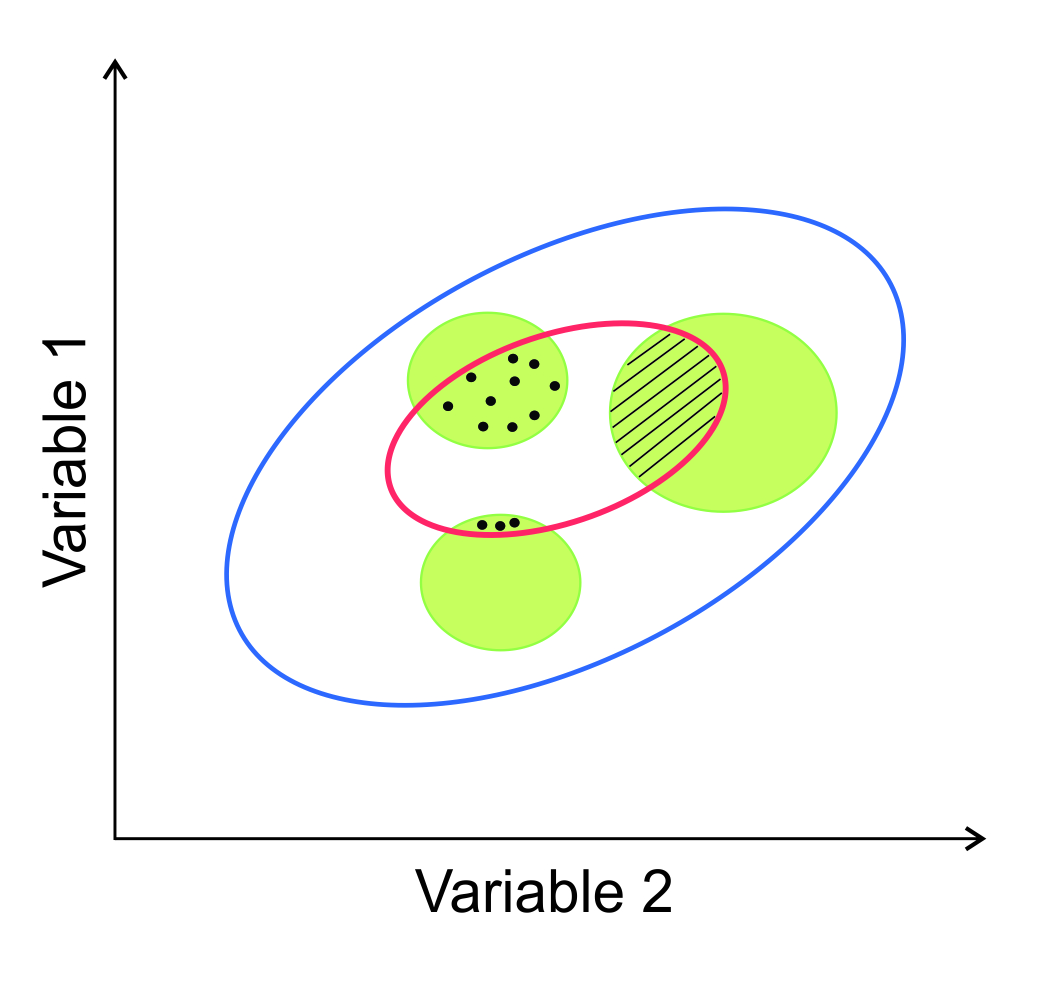
Figure 7.1 Hypothetical species tolerance ranges to two environmental variables. See text for details.

Here, then, is the major problem inherent in the use of geographical presence data to characterise a species’ niche: we are inevitably only observing the realised (i.e. occupied) niche in that region, with its particular range of available environments and its particular suite of interacting species. There is no way of telling how much this realised niche and the fundamental niche differ. And although we can speculate on some of the factors that might influence the extent of the realised niche, and perhaps demonstrate scientifically which factor is likely to be having some effect, there are no easy ways of quantifying their individual, interactive or synergistic contributions. Moreover, we cannot be sure that the realisation of the niche found in one geographic region will be the same if the species is introduced into another region of the globe, with its particular set of environments and its different suite of interacting species. If we make a quantitative comparison between realised niches (for example, in relation only to scenopoetic variables) in different parts of the globe, we must make a leap of faith in considering that they represent similar things and are quantified in equivalent ways. If we conclude that there are different realised niches in different areas (as in a comparison of native and introduced regions), what does this actually mean and is it ecologically of any significance?

If the fundamental niche is what we really care about – because it is the immutable, ideal ecological truth at the heart of what makes a species individual and unique – then how do we contend with the fact that the fundamental niche is ultimately unmeasurable and therefore unfalsifiable? Is the fundamental niche even appropriate material for scientific discourse? To answer these questions, we must not ask whether the niche is a true concept, but whether it is a useful one, and if so, how it can best be utilised. We must also clearly communicate how we conceptualise the niche and for what purpose. Otherwise, readers will get confused if they operate with different assumptions and different goals. Thus, if we are using the concept of a niche pragmatically, merely to better understand the spread of an introduced species, it does not matter that we are assuming a realised niche and cannot possibly interpret the results in terms of a fundamental niche: as long as we are clear and honest about what we have done and the many assumptions that we have made along the way.

For now, we will leave this discussion of niche theory and focus on what ecologists actually do.

7.4 Niche shifts in non-native species

Human-mediated introductions of species to new geographic regions have received a great deal of attention in recent years because of the significant threat they represent to economic, environmental and social values. The pragmatic concerns of invasive pest and weed management dominate many studies. But many ecologists regard introductions as invaluable ‘natural experiments’, from which we can learn a great deal about basic ecological processes (though experimental design issues of replication, randomisation and power tend to be overlooked). These ‘experiments’ are represented by vast databases of geographic occurrences and dates, which are now readily available online and are commonly analysed in attempts to reveal broad empirical principles. Natural introductions, particularly on islands, featured strongly in the early development of ideas on evolutionary theory and population genetics (Baker and Stebbins 1965). From a conceptual point of view, it makes little difference whether the introductions occurred naturally or through the actions of humans. We know a great deal, in terms of ecological and evolutionary processes, about what happens as a species spreads into new regions. But what can we learn from a comparison of the environments that a species evolved in and the environments that it now comes to occupy in far-off regions? Can we predict the latter from the former? And if not, why not? If so, can we use that knowledge to protect biodiversity and natural resources? It is against this background that an interest in niche conservatism, and its alternative of niche shifts, has developed.

Niche theory was originally driven by an interest in community diversity and largely arose from an Eltonian perspective of the niche. The idea that a species had a niche naturally led to a consideration of the consequences of overlap with the niches of other species. If niches overlap, there will be intense competition between the species for certain resources, perhaps leading to competitive exclusion of one by the other. There might, in response to this, be associated coevolution that reduces niche overlap. ‘Niche complementarity’, i.e. niche differences among species, should lead to more efficient acquisition of limiting resources and therefore perhaps higher overall productivity by the community.

Theoretical modelling explored factors likely to drive the evolution of niche differentiation at a local scale (e.g. Roughgarden 1974). On the other hand, species tend to retain ancestral ecological characteristics and evolution often appears to be highly phylogenetically constrained (Pyron et al. 2015). There has been a great deal of debate, for example, over why species are unable to adapt to conditions just beyond the edge of their native range (Hargreaves et al. 2014), why so few species (‘extremophiles’) have been able to evolve tolerance to very extreme conditions (Xu et al. 2020) and under what conditions we might expect fundamental niches to evolve (Holt 2009). It is, then, logical to ask whether or not, in general, niches tend to be conserved when a species invades a new region. New opportunities are often available to the species and existing constraints are frequently relaxed. Perhaps under such conditions niches will be able to shift more readily than they do in their native ranges.

Before we consider the methods that researchers use to draw their conclusions on these questions, it is worth considering what it means when we say ‘niche shift’ in regard to an invasion and some of the jargon that is being used (Box 7.1).

Box 7.1 The new language of invasion ecology

Consider the available environments in a region where a species originally evolved and expanded (yellow region in Figure 7.2a). Part of this overlaps with the fundamental niche (dark blue ellipse) and can potentially be occupied by the species. However, because of limited bionomic variables and the impacts of other species, only a subset is actually occupied (the realised niche, green shaded area). Regions I are too inhospitable for the species to be able to evolve; regions II would be suitable but do not exist. If we were to plot all known occurrences of the species in this graph (often referred to as a map in ‘E-space’, rather than a map in geographic or ‘G-space’), they should all fall within region III.

Now consider that propagules from a population (its tolerance range shown by the small ellipse) at point X in the home region are transported to a new region, whose available environments are shown in pink in Figure 7.2b. The initially suitable scenopoetic range in the new region (small ellipse) may be smaller than that of the source population because only a subset of genotypes will arrive. If the point of arrival is a location with suitable scenopoetic variables, sufficient bionomic resources and tolerable biotic interactions, it can successfully colonise – even though the conditions may be outside the realised niche from the home region. It can then spread and evolve, ultimately being present throughout a new realised niche.

A new set of terminology (Fig. 7.2c) has been coined to distinguish between regions of E-space with respect to niche shifts (Guisan et al 2014):

• Non-analogue environments: environments in the new region that were not present in the native region (that part of pink region of Figure 7.2c which does not overlap with the yellow region).
• Abandonment: occupied environments in the native region that are unavailable in the new region (A).
• Unfilling: environments that were suitable in the native region but not occupied in the new region for some reason (U).
• Pioneering of non-analogue environments: environments occupied in the introduced region that were unavailable in the native range (P).
• Expansion of the realised niche: environments occupied in the introduced region that for some reason were not occupied in the native region (E).
• Overlap (or stability) in the new and old realised niches (O).

   

  

   

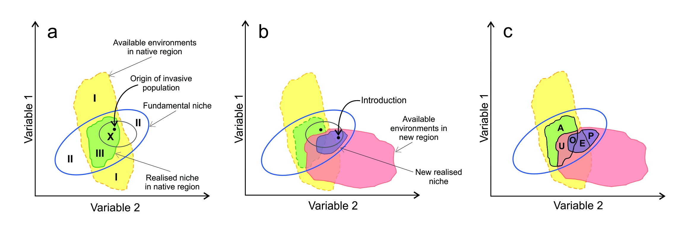
  Figure 7.2 Representation of environments in native and introduced regions, along with fundamental niche and realised niches. Also shown are the points of origin and introduction of the invading phenotypes with their tolerance ranges. See text for details. (c is modified from Guisan et al. 2014.)

7.4.1 The data

If we want to estimate realised niches empirically, we require data on environmental conditions at locations where the species occurs in the native and introduced regions. This requires a number of assumptions. Here, we discuss those assumptions regarding the qualities of the data in databases, addressing sampling issues, conversion of spatial coordinates to environmental variables and the selection of the environmental variables for consideration.

Occurrence records. We usually begin by accessing information on species presence in G-space and then determining environmental variables for those locations. The first assumption is that our ‘presence’ data are reliable and representative of the species niche we are trying to characterise. The vast majority of available presence records come from global databases compiled from information provided by a variety of collectors, such as the Global Biodiversity Information Facility (GBIF: https://www.gbif.org/). Extreme caution is needed when using these sources (Newbold 2010) as little quality control has been performed on the data. Such databases are not primary information and have often been transposed from other sources, and for older records, the exact locations might have been guessed and the taxonomic determination may be outdated or based on features inadequate to determine identity with confidence. Three factors threaten to derail niche estimation at the first step: spatial accuracy, taxonomic accuracy and microclimates not captured by the variables used to define the niche.

First, spatial errors are particularly common in some widely used databases. Older records collected before handheld GPS units were common often had little information on their spatial location. Digitisation of information on the labels of herbarium specimens can also introduce errors, as it is often conducted rapidly, by non-experts and without the funds necessary for high levels of quality control. Sometimes an occurrence may be deliberately allocated to the latitude and longitude of the capital of the country or the country (or regional) centroid, rather than the actual place of collection (Kriticos et al. 2014).

Second, it is common to find errors in identification of the species, even for accredited sources such as herbaria, again with the potential to cause bias (Webber et al. 2011a). Some taxa are inherently difficult to identify, especially if key traits (such as flowers or fruits) are missing and herbaria are seldom able to keep up with all taxonomic revisions; in one study (of sea rockets, Cakile spp.: Cousens et al. 2013) the error in invaded regions was around one-third of samples. Databases such as iNaturalist are now often including samples from unverifiable surveys or from amateurs (‘citizen scientists’). If our aim is to make definitive ecological statements, it is surely essential to have all records verified by an expert in that species. This is rarely done in published studies of niche shifts, simply because of the volume of data. It is, however, becoming easier to conduct some level of quality control, even if accessing data online: many (but not all) herbarium specimens are now available at good resolution online, and citizen scientist records are often accompanied by photos.

Third, and of particular relevance for introduced populations, is the role of microclimate in enabling the presence of a species in a given area. That is, if a microclimate facilitating local persistence is not adequately represented in the environmental variables (generally gridded rasters) used to define the niche, then the resulting niche will be misrepresentative. For organisms that can modify their experienced climatic niche by moving through space or time (animals, dormancy), microclimates (forest understorey communities) or mutualisms (assisted seed dispersal), or for species where inter-annual variation in climate is significant, broad-scale climate averages are largely irrelevant to defining the realised niche.

For example, the issue of resolution and scale is frequently encountered for records that are spatially restricted to riparian environments in arid landscapes, or for introduced populations that rely on localised human landscape modifications (e.g. the watering of seedlings during dry summers) to establish and/or persist (Webber et al. 2011b). Ensuring that the spatial accuracy of presence records accords with the resolution of the environmental variables is therefore critical. Moreover, as we discuss in the section on environmental variables below, this is not an issue that is fixed by simply down-scaling the environmental layer to create a false perception of finer resolution.

All three factors can result in frequent errors in G-space for presence records and thus considerable error in E-space. Data are, therefore, sometimes ‘cleaned’ prior to analysis. The most common cleaning performed is to remove spatial outliers, and procedures are available for automating this process. However, outliers in either G- or E-space may not necessarily be mistakes and in fact can hold useful information about the species (e.g. coastal species spreading through the use of salt on interior road networks). It is straightforward to search for and remove individual records that suggest the species occurs in a highly unlikely place, such as a terrestrial species in the middle of the ocean. Validating taxonomic determinations and correctly identifying microclimate-restricted records is, on the other hand, especially challenging, particularly for older records.

Even if these three factors have been adequately addressed, other cleaning, called ‘occurrence thinning’, may be done to remove multiple records at the same geographic location or in the same grid square. This approach can reduce bias from over-sampling of some regions or environments. Occurrence thinning is often recommended in the literature, and in some cases it does improve outputs, but it exposes a serious issue: as we fiddle with our data (and our models) we obscure our assumptions, in turn obfuscating our ability to make inferences.

In the case of occurrence thinning, the chief assumption is that in grid cells where records exist, differences in the number of records are due to sampling bias and not to ecological differences in abundance, detection probability or habitat suitability. Conversely, it is assumed that ecology – and not sampling bias – is the only thing determining whether a grid cell has any points to begin with. If the downstream goal is to characterise all possible environments a species can inhabit (e.g. with an envelope model), this assumption might be appropriate. If the goal is to estimate occurrence probability or to quantify habitat suitability, it is not at all clear what an occurrence-thinned distribution represents, especially if it is applied to a real-world system where these two assumptions certainly do not hold.

Which environmental variables to consider. Once we resolve the data cleaning issues to our satisfaction and select occurrence data to use, the next step in data processing is to identify the environmental variables we want to use to measure the niche. Numerous environmental datasets, varying in temporal and spatial scales, are now available for different regions and include marine environments (Fréjaville and Garzón 2018; Tyberghein et al. 2011). Continent-wide data, for example, are primarily climatic or related to physical variables, whereas edaphic data (soil type, pH, salinity) tend to be more restricted. Some programs will generate environmental variables based on various future climate change scenarios (incorporating all manner of assumptions; e.g. Noce et al. 2020).

Assumptions are required by the algorithms used in software to generate values of environmental variables at a given set of spatial coordinates. For example, primary environmental observations recorded at point locations - meteorological recording stations – need to be converted to gridded data rasters through some sort of smoothing procedure. This also requires us to assume an appropriate grid size, but different grid sizes will result in different levels of error. While there seems to be a race to produce ever-finer climate data layers (e.g. the WorldClim database now comes in 1 km grids: Fick and Hijmans 2017), there is a real danger in equating greater resolution with improved realism (Daly 2006). For example, given the often sparse density of station point data that underpin climate layers, the excessive precision of finely gridded data layers can lead to spurious conclusions. In turn, inappropriately large grids in areas where environmental gradients are steep can also cause problems. Consider, for example, a large grid size in a steeply mountainous area, for which an ‘average’ environmental value may be highly misleading. We therefore need to match the resolution of the environmental variables chosen to the precision of the occurrence records and the nature of the research question being addressed.

In studies of niche shifts, we are required to assume that the variables used are the most appropriate ones for the species and regions under consideration. That is, either through theoretical framing or experimentally informed decisions we have concluded a mechanistic relationship of some kind between the particular variable and the range-defining factors for the species. But how do we make that decision?

The Hutchinsonian concept of the niche considers environmental variables that directly impact on the life of an organism, such as temperature and humidity. There are programs – again incorporating various assumptions – that will generate physiologically relevant variables anywhere on earth and even the metabolic rates for the species (Kearney and Porter 2020). However, most niche shift studies rely on a set of variables, referred to as ecoclimatic, bioclimatic, climatic or more prosaically ‘Bioclim’ variables (after the program that made these widely accessible; Booth et al. 2014). Indeed, the term ‘climatic niche’ is now used in many studies: the availability of data is driving our concept of what the niche is!

Instead of being the environmental factors experienced by the organisms at a given point in time, these bioclimatic variables are often assumed (implicitly or explicitly) to be environmental surrogates that are correlated with proximate drivers of the distribution, such as annual mean temperature, annual precipitation and seasonal patterns such as the mean temperature of the wettest quarter. In some cases, ecological theory or experimental evidence is used to support this choice of variables, which has driven an increasing focus on variables that capture extreme conditions rather than average conditions. There is also a need to make assumptions about the most appropriate time window over which to generate bioclimatic variables. As a result of climate change, it is possible that the data no longer apply to a given location and an element of bias may be present, particularly if there is a mismatch between the temporal windows over which bioclimatic and presence record data have been gathered. For this reason, some researchers now restrict their data sets to averages over only recent decades and avoid using historical presence records.

The use of simplified surrogate variables assumes that the surrogate has a stable causal connection to the actual variable driving species distribution for the time and region under consideration. If this assumption is invalid, inference is dangerous. For example, in one region a short-lived species may find the appropriate conditions at one time of year (e.g. autumn), while in another region it may find those same conditions at a different time (e.g. spring). Two regions may share a similar climate, but the species may only occur in one of them because they require a particular range of soil pH or drainage (the importance of the edaphic environment has long been appreciated by phytosociologists; e.g. Ellenberg 1974).

Which of the many climatic variables should we then use? The WorldClim database, for example, provides 19 variables (Fick and Hijmans 2017), while the CliMond database provides 35 variables (Kriticos et al. 2012). In the early days of the analysis of species distributions, researchers chose as many variables that appeared to align well with geographic limits, such as some temperature at a particular time of year. Many researchers chose to throw all variables at the model in the hope that something would stick. If we have many covariates readily available, it is tempting to use them all (we will return to this issue later in regard to species distribution models). Some of them may be effectively redundant for the species/region under consideration and there may be high levels of correlation between variables, both issues leading to statistical issues in any subsequent calculations.

Many niche shift researchers allow the data to tell them what is correlated, by using principal component analysis (PCA) to reduce the dimensionality of the data from n variables to just a few composite ‘climate’ axes (sometimes only two). This also allows the results to be presented visually (see Figure 7.3) and facilitates comparison of native and non-native range data. While in some ways it is useful to distil data down in this way, any simplification discards a considerable amount of information on environmental differences among locations. This is a problem if the proximate ecological drivers are not correlated with the composite variables that are retained, and an even greater problem if the proximate drivers have correlations with the causal variables but these correlations differ between the native and non-native range. Ecological interpretation of composite variables is challenging at best – yet another assumption that we choose to make – and composite variables do not transfer well into other regions or across studies. Finally, PCA involves correlations among the predictor variables, but we are often more concerned with covariation between predictors and species occurrences. When we do PCA and cluster the most tightly correlated predictors, we should not assume that these are also the most effective predictors.

Once we have chosen the environmental variables we will be working with, the next step is to convert the spatial coordinates (in G-space) to environmental coordinates in the E-space we have just defined. This process is called ordination and it is as simple as plotting the environmental values for each occurrence in E-space. We now have a cloud of points in E-space representing occupied environments in the native and non-native ranges.

Box 7.2 The use of composite axes to determine niche overlap

A word of warning is necessary regarding the common practice of collapsing clouds of multivariate points on to just two composite axes, prior to comparison of native and non-native niches.

While environments are multidimensional, it is much easier to think of data if we can depict them in a simple, two-dimensional graph. There are multivariate statistical methods which do this very effectively, such as principal component analysis: they allow us to reduce the number of axes, but at the same time retain as much of the original information as possible. Thus, 20+ independent environmental axes might be reduced to just two or three composite axes and retain, perhaps, 60–70% of the variation in the data.

An example is given in Figure 7.3. Occurrences of Cakile edentula (in native (green) and two non-native (blue) ranges are plotted against the first two axes from a principal component analysis of 19 bioclimatic variables. The large empty region within the native polygon shows climates that simply do not exist in eastern North America. In the non-native ranges, there has been both a shift in the centroid and an expansion of the E-space occupied. According to standard methods of analysis of climate niches this would constitute a shift in the ‘realised niche’ of the species. A plausible explanation for the shift is that it is the result of a very broad innate climatic tolerance of the species and highly restricted available combinations of climate in each region. This is supported by the ability of native range genotypes to establish in non-analogue climates (two of the three white symbols). Although other research has shown that adaptation by C. edentula in new locations has occurred, that may well not be the reason for a shift in the realised niche.

 

 

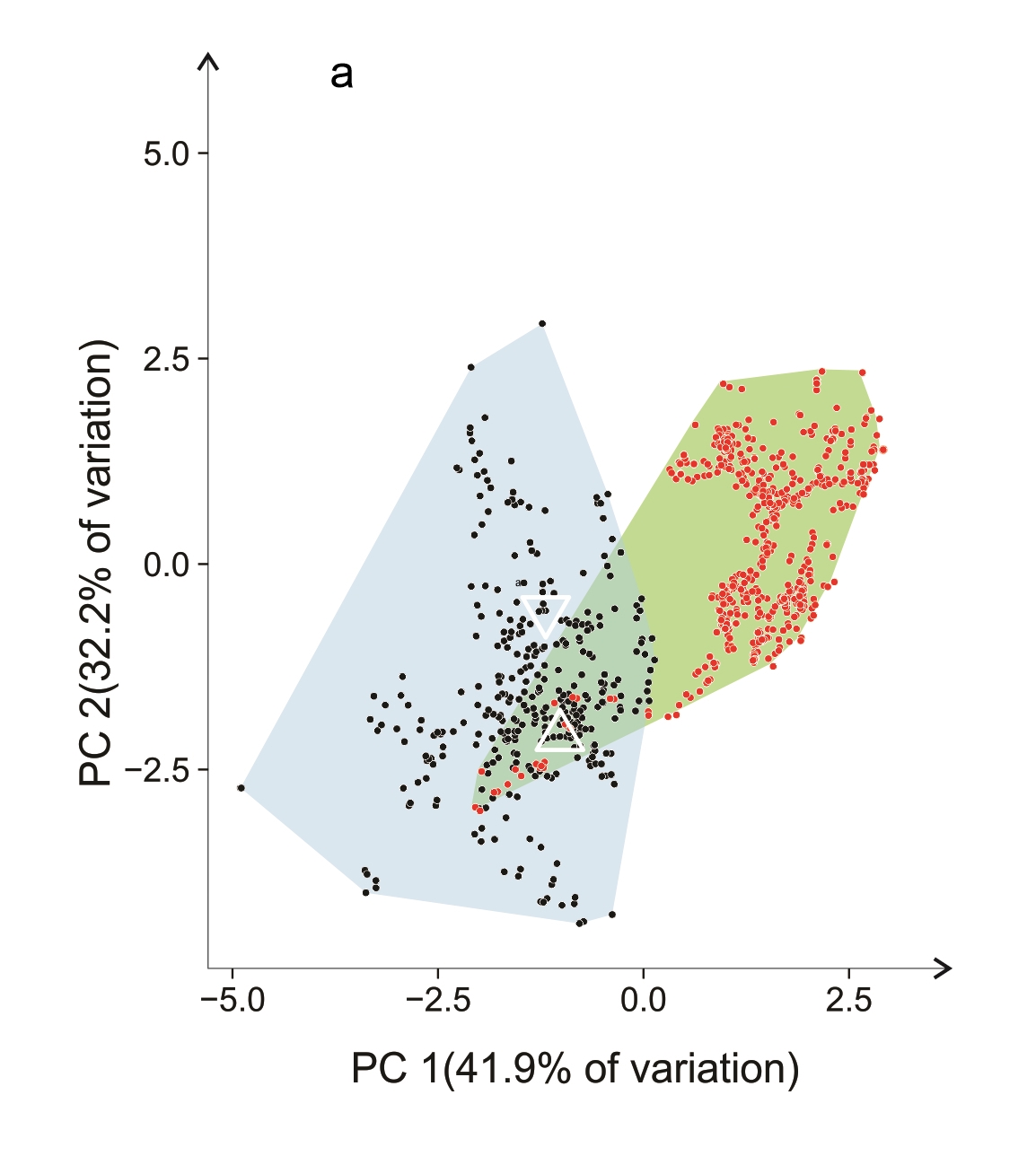
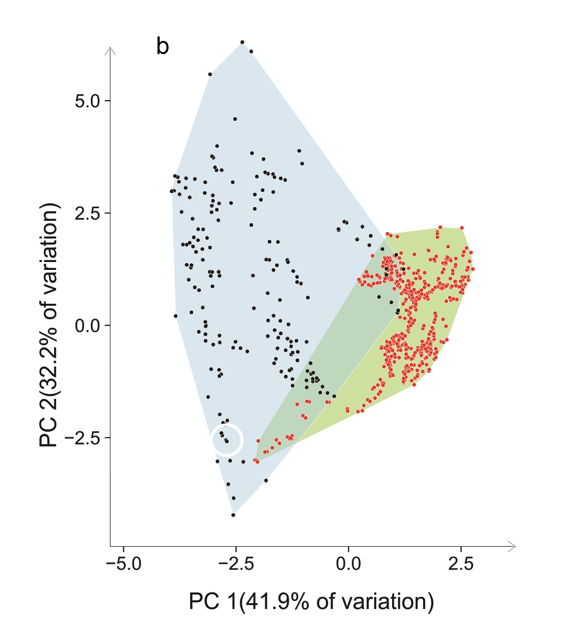
Figure 7.3 PCA ordinations of Cakile edentula in native (red dots, eastern North America) and two of their non-native ranges (black dots): (a) Australasia, (b) western North America (courtesy Philipp Robeck). Data were sourced from GBIF (https://doi.org/10.15468/dl.yc5cxc). Records from non-native regions were checked visually to confirm the species and incorrect records discarded. White symbols indicate first non-native records: Δ Australia; ∇ New Zealand; Ο western North America.

The use of two-dimensional ordinations, however, can cause serious misinterpretations of niche overlap. It is highly likely that clouds of points that have no overlap whatsoever in multiple dimensions will appear to overlap in two dimensions. Just imagine being in a three-dimensional world and taking two-dimensional photographs of two balloons, flying separately. From some directions, a 2D image would look as if the balloons overlap, but they do not in the real 3D world. How many of the cases of apparent niche overlap in the literature, based on analysis of PCA data, are actually false?

7.4.2 The analysis

At this stage, our goal is to measure whether a niche shift has occurred, by comparing the native- and non-native-range data sets we have gone through so much trouble to create. We need to assume that each of these clouds of points gives an adequate description of the n-dimensional space potentially occupied by the species in each region (see Box 7.2).

There are many difficulties with this assumption. Firstly, unless we set out to evaluate the dynamics of invasions, such as the lengths of lag phases, we must be prepared to accept that each species has managed to access all suitable environments. While this might be reasonable for the native region, where dispersal has been able to take place over millennia, species in introduced ranges may have only had opportunities for a matter of decades or a few centuries at most. Can we be sure that the species has stopped spreading (Forcella 1985), when we know that lag phases can be common and potential environments may extend over thousands of kilometres, or where sharp geographical barriers exist (e.g. steep mountain ranges)?

Secondly, we know that the distribution of data from databases within E-space can be very uneven, which potentially biases subsequent analyses (Meyer et al. 2016). Sampling bias in E-space comes from two sources. Environmental sampling bias occurs when certain environments are more common than others, creating hotspots in E-space. Geographic sampling bias occurs when certain locations are more sampled than others. Sampling bias can easily result in a change in the location of the centroid of the data (a common measure used for niche shift), without there necessarily being any change in the niche at all.

While there are ways of trying to remove such bias and for smoothing data (Atwater et al. 2018), these methods have their own assumptions and are unlikely ever to perfectly overcome the issue. Nonetheless, removal of sampling bias is absolutely vital. If there is bias in either of our clouds of points, then there may be bias in our conclusions about niche shifts.

Finally, there are a range of other sampling problems subsumed within the data. For example, is the sample size sufficient for a good representation of the entire environment space in all of its dimensions? The extremes of distributions may be poorly recorded due to the rarity of the species, leading to an underestimation of niche overlap or niche shift. Because we rarely have accurate estimates of geographic sampling bias, we may be tempted to throw up our hands and ignore the issue. However, it is important to keep in mind that every decision we make involves a commitment to certain assumptions (see also Box 7.3).

If we decline to address geographic sampling bias, we are committing to the assumption that every region of our study area has exactly the same sampling effort. If we decline to address climatic sampling bias, we are assuming that no environments are more common than others. Because these assumptions are likely to be far removed from the truth, we must challenge ourselves to do better.

Calculating the niche and niche overlap. The cloud of occurrence records in E-space may expand, contract or remain unchanged from the home region to the introduced region and it may or may not move its location. There are various ways of summarising clouds of data points mathematically so that their properties – and any change in those properties – can be analysed; each has its own assumptions. We consider three approaches here.

First, we might measure the volume of the cloud of points by establishing a boundary (such as a minimum convex hull or contoured spline) around each data set and then assess the degree of overlap of the hulls in some way. This assumes that the outermost points represent the maximum extent of the species and that the edges of the polygon introduce negligible error. It is essentially the same approach used by Hutchinson (1978; Chapter 5). Second, we might assume that the niche has a given statistical distribution (e.g. elliptical) across E-space and then compare the home and invaded distributions in an appropriate way (e.g. Guisan et al. 2014). Third, we might calculate some sort of index of overlap based on grid cells in E-space that contain occurrences from one or both clouds (e.g. Schoener 1968). Again, we assume that the index is a valid estimator of overlap.

To compare two niches, however defined, some metric of difference is used. There are many possible indices, each likely to have different sensitivities to the distribution of data, and the options are restricted by the method that has been used. For example, with hulls and contours we can compare areas of overlap (Petitpierre et al. 2012). With any approach it is common to calculate the positions of the centroids of the clouds, in order to measure the direction and magnitude of any niche shift rather than just whether or not it occurs. This assumes that the centroid, an arithmetic mean of the data, is an appropriate summary of the data. It is possible for there to be a significant change in the centroid without there being any change in the overlap of the clouds of points, so other metrics are also needed, each with their own set of assumptions.

The final step is some sort of statistical analyses of the data. Commonly this is a permutation test, involving resampling of the data clouds and the construction of a probability distribution for the estimated difference being simply the result of chance. Such tests are, in themselves, highly robust and avoid problems that can be introduced when using parametric statistics. Following these tests, we need to make a binary decision about whether or not the probability is low enough that we can safely conclude that the difference is real (statistically ‘significant’). It has become traditional in ecology to use a cut-off probability of 0.05. This is another assumption, that this high and entirely arbitrary level of confidence is an appropriate default threshold.

Box 7.3 Take care with software

A word of warning is worthwhile in relation to the use of user-friendly or semi-automated software for research on this topic, on SDMs and in research more generally. Most software assumes, implicitly, that the user knows and understands what they are doing when they parameterise their model and produce outputs, that the issues they are exploring are appropriate to address with this method, that they appreciate potential issues with their data, that they have taken appropriate remedial actions and that they are appropriately interpreting the outputs. If remedial actions are included as part of the package, they are usually options that the user needs to make a conscious decision to select.

A real possibility is that casual users, who are unaware of the potential pitfalls, will use the package with default settings unchanged, producing results that will look (at least superficially) appealing and may make some sense, but yet are not actually appropriate. Default settings may cause the user to overlook important departures from the assumptions of the methods. It is left to the researcher and the reviewers of their papers to know what to look out for – which will not always be the case. We will return to this issue when we discuss species distribution modelling.

7.4.3 Interpretation

We now reach a point at which we interpret our results. Has there been a shift in the realised niche? We start with a word of warning – one that applies not just to niches, but across any science using statistics. The search for evidence of whether or not there are niche shifts may lead some researchers to interpret non-significant results as instances of no difference between the clouds of points. This is unwise. From a logical viewpoint, absence of evidence is not the same as evidence of absence. ‘Non-significant’ only tells us that, to the high levels of confidence that we have set, we do not know whether there was truly no difference in the calculated metrics or whether the data were simply too noisy to be able to tell (see Chapter 4). As a result, false negatives will strongly bias a conclusion towards an absence of differences.

It is common to conduct niche shift analyses for many species in order to draw conclusions on the generality of a niche shift. If one or other outcome is more common in a meta-analysis, then we accumulate support not just for the fact that niche shifts can occur (or seldom occur), but that they are common (or uncommon) enough that there may be a fundamental ecological principle behind the results. A finding that niche shifts for non-native introductions are common (or, alternatively, that they are rare) could be considered to be a robust conclusion: despite all of the assumptions and all the uncertainties about the data, the same result is found for a great many species in a wide diversity of environments. So, the evidence seems compelling. However, it could be that bias in the data is extremely common, making it more likely than not that an apparent niche shift would be found – but which would, in fact, be an artefact.

A spanner in the works, however, is the fact that the qualitative outcomes of studies vary. Some studies have announced that niche shifts are rare or often unable to be detected (Guisan et al. 2014), while others have concluded that they are common (Atwater et al. 2018). Can both conclusions be true? Perhaps it is the differences in the methodology between the studies that resulted in the difference in conclusion (Webber et al. 2012), or the selection of species. Such conflicts in conclusions are of concern. How do we resolve them? Do we accept the most up-to-date study using the most advanced methods as being more likely to be true?

But how do we know, for example, that newer methods have not introduced new invalid assumptions that bias our conclusions? The statistically significant positive conclusion of a niche shift (or the conclusion of no evidence of a niche shift) may still be false – because the data do not fulfil the many assumptions that we have made about them, the data cleaning may not have achieved its aims, our assumptions in the choice of variables were wrong or our calculations of overlap may have been inappropriate. Perhaps we might need some sort of independent forensic analysis of the conflicting studies with respect to the validity of the assumptions and the properties of the data. Even then, after consuming countless hours of effort, we suspect that no unequivocal conclusion would be reached.

Comparisons of climatic environmental data in two regions are regularly used to indicate some of the things that may have happened to cause a shift in the ‘climatic’ niche (see Box 7.1). Some of these are particularly useful for excluding niche shifts that may well be geographic quirks: chance differences in availability of environments in the two regions. Unfilling (Box 7.1) – a failure to have (yet) occupied apparently suitable environments in the new region – was notably frequent in Atwater et al.’s (2018) study at a continental scale (Figure 7.4). This might not indicate a fundamental niche shift in any ecological sense (just a time lag as an invasion proceeds), but unfilling will have a considerable effect on the centroid and range of a set of points in E-space and make it more likely that a niche shift will be calculated. Abandonment – the mere unavailability of suitable climates from the native range – was also strongly represented in the Atwater et al. data: in other words, the apparent shift in the niche is heavily influenced by a change in climate availability, and not necessarily by a change in the fundamental niche of the species.

 

 

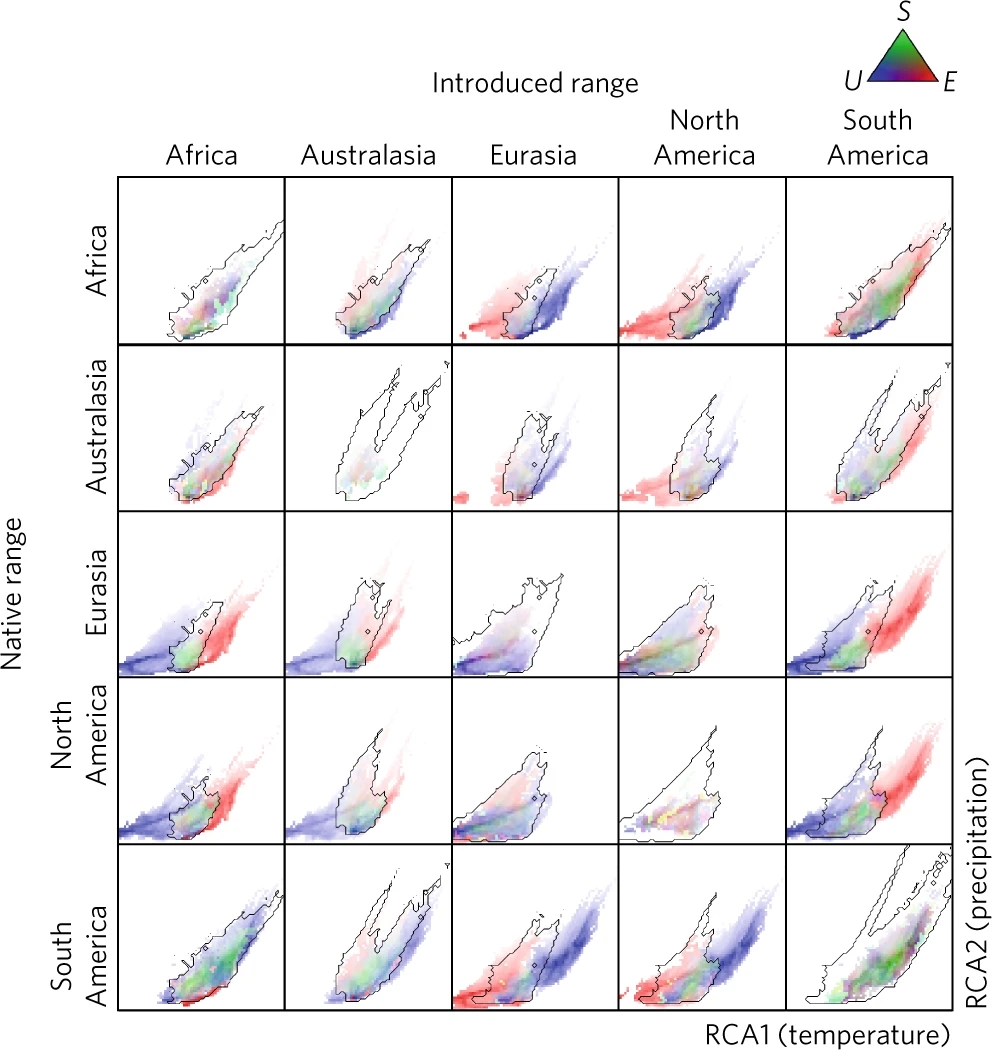
Figure 7.4 Principal component analysis (PCA) comparisons of occupied climates in 815 plant species in their native and non-native range (first published by Atwater et al. 2018). Environmental data were rotated to fall along two axes: an axis indicating increased temperature (RCA1) and precipitation (RCA2). Black line shows climate space in common between native and invaded regions. Blue points inside analogue space represents ‘unfilling’; blue points outside analogue space indicate ‘abandonment’. Red points inside analogue space represent ‘expansion’; red points outside analogue space represent ‘pioneering’. See Box 7.1 for definitions of these terms. Green points are ‘stability’ (similar climates occupied in both regions).

Whatever the analysis has been, we must make a final judgement that a shift in the realised niche actually means something ecologically. Or that it tells us something that is useful in a practical sense. As we discussed in The Niche Concept Meets the Real World (this chapter), there are several reasons why a difference in realised niche might occur.

It may be due to the differential geographic availability (and accessibility) of suitable habitats in the two regions – into which the species can ‘shift’ because of its inherent tolerance (not to be confused with phenotypic plasticity; Lande 2014) or because it undergoes local adaptation. It may be because of unspecified differences in the biotic environment, bionomic resources and their interactions in the two regions.

It could be that for some reason the species extends its fundamental niche in the new regions (which begs the question of why it did not do so in the native region, so is this a realistic expectation?). It could be a combination of all these things. How can we tell which? There is no simple answer. For example, there will always be differences in the biota in geographically remote regions: this underpins the often-tested enemy release hypothesis explaining the success of biological invasions (Keane and Crawley 2002). How can we tell how much impact these factors have on the realised niches and their overlap? It is common to find evidence that there has been local adaptation in the new region (e.g. van Boheemen et al. 2019), but we expect local adaptation to occur in the native region and within the fundamental niche. Adaptation, of itself, is not necessarily evidence of a niche shift.

7.4.4 Uptake of conclusions by others

As discerning scientists, we should always be aware of the assumptions that a study has made and treat the results with the appropriate caution. If the study is someone else’s, we must not ignore the ‘fine print’ – though experience is needed in order to know what to look for, particularly when the fine print is missing. Weakly supported assumptions can only result in weak inferences and it is poor science to perpetuate these.

In the context of niche shifts for introduced populations, we have reviewed the considerable number of assumptions that need to be made in drawing conclusions from location data. The data that are commonly used for these analyses are known from the outset to have many problems that make them in many ways inadequate. Yet, authors commonly make bold statements about what they have demonstrated, while papers by other authors referring to the results readily accept those bold conclusions at face value.

As an example, consider Atwater et al.’s (2018) paper analysing data on 815 plants which stated boldly in its title that ‘climatic niche shifts are common in introduced plants’. If we read the detail in the paper (the fine print), we find many caveats recognised by the authors. The paper also relies on a number of assumptions not detailed explicitly in the paper. Many of the assumptions relate to the reliability of geographic presence data from a restricted range of environments in order to make statements about the species’ tolerance to all possible environments. Unfilling – resulting possibly from a failure to have (yet) occupied apparently suitable environments in the new region – was notable in Atwater et al.’s study at a continental scale. Abandonment – the mere unavailability of suitable climates from the native range – was strongly represented in the data (Figure 7.4). In other words, the apparent shift in the niche may have been heavily influenced by dispersal limitation, and not necessarily by a change in the fundamental niche (or strict-sense realised niche) of the species. Tellingly, Atwater et al. (2018) were pressured to remove a more nuanced discussion of these issues by reviewers who found it uninteresting.

In another example, ‘Most invasive species largely conserve their climate niche’ was used as a headline by Liu et al. (2020) – the opposite conclusion to Atwater et al. – even though these authors stated in the text that the work had ‘two important caveats’ (one of them related to the meaning of the realised niche). Interestingly, these conflicting accounts often rely on the same data. Where they often differ – as between Atwater et al.’s (2018) account and Petitpierre et al.’s (2012) – is in how the data are handled, and in particular what assumptions are made about sampling bias.

The greatest message from this work may be that the conclusions we draw depend heavily on the assumptions we make, but disentangling these issues requires deep, working knowledge of the subject area and particularities of model implementation that is inaccessible to almost everyone, sometimes including the authors themselves. No wonder, then, that readers have so much trouble interpreting the conclusions that have been made!

We examined 67 citations of Atwater et al.’s study. Of these, 63% of papers cited the study as conclusive evidence that niche shifts exist and are common, with a strong implication that this tells us something significant about the biology of the invading species (rather than just about the environments on offer). The reviewers and the editors had accepted these opinions of the citing authors (or the rights of the authors to state them). Most papers (94%), however, made no mention of the fact that the study only tells us about the realised niche. The reported niche shifts were sometimes considered by the citing authors to be the result of phenotypic plasticity or tolerance, but also alongside adaptation: 10% of citing papers used the paper as evidence that selection, adaptation or evolution occurs during an invasion, even though there is no logical basis on which to draw such a conclusion. Just one paper questioned what a shift in a realised climate niche actually means, while one other paper used it to draw attention to the importance of unfilling as a component of apparent niche shifts. It is not difficult to see how a process akin to ‘the telephone game’, i.e. cumulative errors, can enter ecology and be detrimental to syntheses of results.

7.5 Species distribution models

Not all ecological analyses of species distributions have the niche per se as their focus. The end goal may, instead, involve some quite mundane statement about the species’ geographical range: for example, we may want to know where to search for unknown populations of a rare species (e.g. Maycock et al. 2012) or how widely a species may spread when introduced into a new region. From this, we might be able to draw implications of various forms of management options or to calculate some measure of persistence likelihood or introduction risk. We collect data on species geographic occurrences, use this to make a model of the species’ known distribution in E-space and then project it back into G-space (Figure 7.5). This type of model is called a species distribution model (SDM), otherwise known as a habitat distribution model (HDM) or more generally as a type of ecological niche model (ENM), and it represents a hypothesised species distribution. Since many studies consider only climatic data, SDMs are sometimes referred to as climate matching or bioclimatic models (Sutherst 2003). Terminology remains inconsistent and often confusing. However, by far the most common type of SDM is built by correlating occurrence data with environmental data. Some SDMs also use absence data, where available, or surrogates for absence (pseudo-absence data, backgrounds), which also come with their own set of assumptions and potential pitfalls.

While the study of niche shifts for introduced species does not necessarily involve correlative SDMs, and SDMs can be used for the study of issues other than biotic invasions, the two topics have much in common. As a result, studies of niche shifts and species distributions share many assumptions, but SDMs also introduce new assumptions related to the ways that data are used. Over a few decades, correlative SDMs have become a standard research tool for many ecologists, but not all of them are necessarily familiar with how the methods should be applied (Lowry et al. 2013). Increasingly widespread, user-friendly software also introduce variability in application, output and user expertise (see Box 7.3). Papers describing and comparing the various methods have achieved huge citation rates (Peterson and Soberón 2012), reflecting their popularity. By 2011, SDMs were included in around 1000 scientific papers per year and these volumes do not seem to be declining. It has become common, for example, for an introductory chapter of an ecological PhD or MSc thesis to include the results of an SDM of the study species. Free, menu-driven software (e.g. Phillips et al. 2017) make SDMs available and easy to use, but also an incredibly easy way to make mistakes (Yackulic et al. 2013).

Here, we will deal with three types of issue specific to SDMs: the assumptions and performance of different models, the training data that are used on a case-by-case basis and software implementation issues. We caution that there are many more assumption-related pitfalls that can impact SDMs but these are beyond the scope of this summary.

 

 

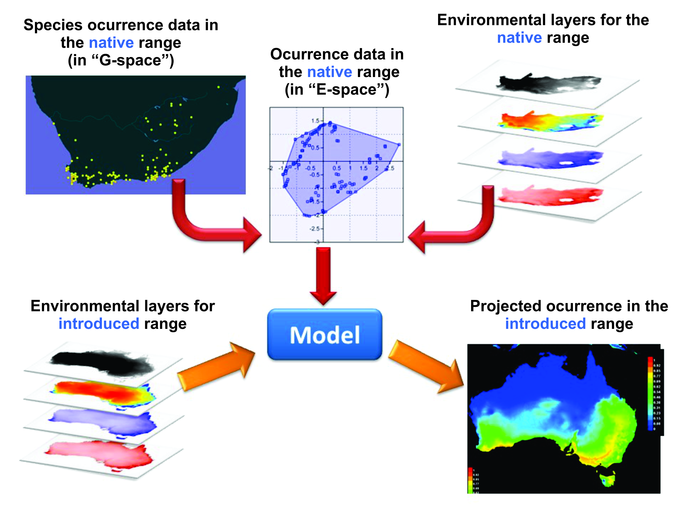
Figure 7.5 Principles behind correlative species distribution models and their use for projecting the eventual ranges of introduced species. Example is for a native of southern Africa that has been introduced into Australia. Figure courtesy M. Mesgaran. See text for details.

7.5.1 Choice of model

There are many correlative SDM methods available: Elith et al. (2006) divide these into envelope methods (mirroring Hutchinson’s original concept of the niche, such as BIOCLIM), regression methods, machine-learning methods (including the most commonly used Maxent) and dissimilarity methods. They all go about their tasks in different ways and make different assumptions. The reason we have so many different SDMs is that there were obvious weaknesses in the early approaches, researchers were starting to ask different questions of the models and improvements were sought. We will not go into a detailed exploration of each approach here; there are excellent guides already published.

Basically, geographic occurrences are converted into points in E-space using appropriate software or environmental layers for that region (Figure 7.5). These are used as input (as ‘training’ data) for the parameterisation of a model that then makes a projection to the same or another geographic region (in the case of Figure 7.5, Australia). As noted earlier, some methods use known absences (or other surrogates of absence) as well as known occurrences. Note that we often refer to ‘projections’ rather than ‘predictions’: see Chapter 8 for a further discussion of the strict difference between the two. When applying a model to novel conditions in space or time relative to those in which it was parameterised (e.g. climate change scenarios, non-native regions), the output relies heavily on assumptions and cannot be tested in the near term with independent data, and therefore is a projection rather than a prediction (the latter of which can be assessed using independent data; Keyfitz 1972).

So, which SDM should we choose? This decision can make a considerable difference to the predicted or projected geographic ranges: outputs from different models can vary considerably. If we assume that model choice is unimportant, then we might be making an important error. While it has been concluded that machine-learning methods and other nonparametric approaches often ‘out-perform’ older SDMs (Elith et al. 2006), the difference in their outputs depends on the data set and the objective of the research. If they are all used on the same input data to describe the native range of the species (and if the data are well-suited to the task), differences in outputs among SDM methods may be quite subtle and unimportant from a practical viewpoint. If the data depart from the ideal (even after cleaning and screening procedures) then the differences between model outputs can become appreciable.

Logically, we should choose a model that is appropriate for our particular situation, to minimise model-choice problems. This requires considerable familiarity with a range of models, which only expert users develop. It can be difficult to master the idiosyncrasies of every method so that we use them all properly and to their maximum effect, so that we make the best choice.

Most SDM users work with only a single SDM package, simply because they are familiar with it, its software may be user-friendly and advice is readily available from colleagues. If a method is widely used, surely this indicates that the method must be widely applicable and reliable? Not necessarily! Popularity does not mean that a method is the best – or even adequate – for every situation. Indeed, this rationale for model choice creates a real danger that the model will be used in situations where it is not (the most) appropriate. And there is a strong likelihood that it will be misused for other lack-of-familiarity reasons, as we will see below. Despite all the published comparisons of methods showing that on certain types of data Maxent is one of the better methods, it is probably the most widely used SDM simply because of its accessibility and ease of use. And perhaps for the same reasons, also the most widely misused.

As an alternative to choosing a single method, some ecologists recommend an ensemble/consensus approach, running several SDMs on the same data and then subjectively considering their similarities (Hao et al. 2019). However, it would seem to be inadvisable to include in such a consensus any models whose assumptions are clearly violated or which is known for its consistently extreme outputs (see also Kriticos et al. 2013). The latest version of this approach is to convert the outputs of multiple models to some common currency and render one ensemble prediction or projection, often weighting models based on performance metrics (e.g. Thuiller et al. 2009). We have encountered both continuous outputs (which produce some continuous metric of habitat suitability) and threshold outputs (which produce a binary occupied/unoccupied map) being created in this way. Interpreting Maxent outputs is already troublesome because it produces frequently misinterpreted estimates of ‘habitat suitability’ rather than occurrence probability (Royle et al. 2012). Interpreting ensemble outputs is exponentially more difficult because model averaging obfuscates what the data actually mean. Moreover, the average of many bad models is still going to be a bad model. Greater effort put into carefully parameterising and interrogating a single SDM is likely to produce far more robust results.

7.5.2 Training data

In the section on niche shifts, we dealt at length with the many assumptions that we make of the data that we subsequently use for SDMs. Several points are worth repeating or expanding, as they have been explored at some depth in the SDM literature.

All SDMs assume that the data used in their formulation – the training data – are reliable (free from significant errors), appropriate for the purpose and sufficiently numerous for accurate model calibration. SDMs assume that occurrence data are independent, random samples from the species’ distribution with respect to the relevant environmental variables (i.e. within E-space) and that the niche has been adequately sampled with respect to the n dimensions under consideration. Such assumptions are explicit, statistical and clearly governed by the SDM being used. We tend to give the most attention to such explicit assumptions, yet for them to run ‘well’ SDMs also require a number of implicit assumptions about the overall quality of the data. For example, they also assume that the species is in equilibrium with its environment and that it has reached all areas within the region that are suitable for them to persist: more a potential distribution than an actual distribution (Guisan and Thuiller 2005; Elith 2017). It is possible that a species no longer exists at some former locations: perhaps climates have changed or the species was unable to persist there, even though it was found alive in the past. We tend to assume implicitly that such issues are minor. Another implicit assumption is that selection in the home region has produced all possible phenotypes of which the species is capable and that these are either represented in the sampled data or will be readily selected for in a new region.

If there is a significant departure in any of these assumptions, then model projections could be unreliable. Some assumptions, however, are more important than others. Sampling distribution is one of these assumptions (Phillips et al. 2009; Elith et al. 2011; Elith 2017).

There may be instances where fewer than 15 occurrences give reasonable model outputs (van Proosdij et al. 2016), but such a small number is unlikely to be reliable if they fail to represent the full range of the relevant niche variables, or if there are a large number of predictor variables. Wisz et al. (2008) recommend a sample size of at least 30 for adequate power. Unfortunately, we may not know what is adequate until data have been collected. Some SDM methods are relatively robust to outliers but others are not; methods for removing outliers statistically are included in some software packages. But why should outliers be removed if they are valid records?

Another implicit assumption that is often overlooked is that the niche is not ‘truncated’, meaning that the environmental niche of a species is constrained by its ecological tolerances – and not dispersal barriers – on all edges of its distribution. If a species is endemic to southern portions of the main island of Japan, we might think we know a lot about the conditions of its northern range limit, but we cannot know if it could survive in climates warmer and wetter than those encountered in the southmost portion of its range. The niche would be said to be truncated at the southern end. Importantly, truncation occurs in multivariate space, not just along environmental axes. Our imaginary species may actually tolerate cooler temperatures than it encounters in its northern range edge, provided that there is enough rainfall, or it may tolerate greater aridity if the temperature is right, but those combinations of climates that would allow it to extend its range do not exist in or near its current distribution. Thus, the niche can be truncated even if it appears not to be.

Truncation may not cause major problems if the model outputs have the same spatiotemporal parameters as they were trained in. However, the goal with an SDM is often to project into new places and/or times. If the new region has conditions, or combinations of those conditions, that were not present where the SDM was trained (i.e. non-analogue climates, see Box 7.2), the SDM will extrapolate unpredictably and the modeller will be none the wiser. This is the reason it is often recommended to pool a species’ entire global distribution (including the non-native range, if there is one) when training an SDM. However, pooling relies on the assumption that species niches are stable and do not shift realised niches among continents.

Certain SDM techniques are then left to process conflicting information between continents in regard to occupied and unoccupied E-space. If the niche does shift, then the pooled model is specious because it does not represent any niche the species actually occupies! Again, the modeller is trapped in a tangle of assumptions from which there appears to be little hope of escape.

The assumption by far the most discussed in the SDM literature is that of bias in data collection. It is common for some regions of the species’ niche in E-space to be less well sampled than others or not at all. Some regions, for example, are more accessible than others (correlated with particular environmental conditions; see also Syfert et al. 2013 in regard to proximity to roads) while there may be sociopolitical constraints to data collection in some regions. Methods have been developed for ‘cleaning’ the data (Zizka et al. 2019) and, to the extent to which this is possible, to adjust for bias due to clumping of data in some regions of E-space.

One source of bias that is impossible to adjust for is the absence of data from regions of the species’ E-space that is within the innate tolerance of the species but from which the species is currently absent. When we extrapolate from our calibrated models, into non-analogue environments, it would not be surprising if errors in projection were to occur for such reasons (Elith et al. 2010; Elith 2017). Islands, and even continents, where the species occurs naturally simply do not contain all of those environments, or the species has been unable to reach there, or perhaps there are un-modelled variables that preclude their occurrence (such as interactions with other species); hence, there are no data to adequately calibrate the model for other regions. Many SDM users, however, appear to be happy to make the assumption that realised niches in the native and non-native ranges will be identical, despite the high frequency of apparent realised niche shifts (Atwater et al. 2018). Is this wise? If not, then we really should not be using SDMs for this purpose!

Ideally, we would have just as much information about where species are as where they are not. Yet, when recording a species’ observation, people rarely note what species they did not see. This causes a problem, because if our data suggest that a region lacks occurrences, we cannot tell whether the species does not exist there, or whether it exists there but has never been looked for (or found). To get around this problem, some SDM procedures allow users to specify ‘pseudo-absence’ or ‘background’ data, as surrogates for that missing information. To be effective the distribution of the background data must resemble the actual sampling effort: in other words, it should correspond to how hard a species was looked for throughout the area being studied. If not, any biases or errors in the background will automatically – and undetectably – transfer to the final SDM.

The simplest approach is to assume that sampling effort is even, in which case background points are randomly selected with equal probability everywhere. In effect, the uniformly distributed background data tell the model that a species was equally likely to be observed everywhere, and a low density of occurrences can only mean that a species is rare. Unfortunately, where geographic sampling bias exists (and it usually does), an SDM based on such background points will underestimate occurrences in remote places and overestimate occurrences in heavily sampled places. On the other hand, if researchers know that more populated areas are better sampled, they might estimate a sampling bias distribution and randomly sample background occurrences from that same distribution. This approach might produce more accurate models if their assumptions are good, or it might amplify problems if their assumptions are bad. The problems compound if approaches such as occurrence thinning are used: such data processing obscures underlying assumptions about the distribution of the occurrences, making it unclear how those assumptions interact with assumptions made about the distribution of the background points.

If we cannot track our ever-increasing list of assumptions through our chain of modelling decisions, we lose sight of what, precisely, our SDMs represent, and they become functionally uninterpretable despite producing pretty maps.

A final point on the use of occurrence data involves the confidence with which we accept projections that clearly include regions of extrapolation outside the range of the input data. While we can make projections for the changes in species distribution that would result from (hypothetical) changes in the spatial distribution of climate using a space for time substitution, we cannot validate them until enough climate change has occurred so that we can compare before-and-after maps. Nevertheless, we produce such outputs because we consider that we need to. We must, however, be circumspect with regard to the conclusions that we reach.

We have made a best guess of what would happen to a species under conditions that are themselves a best (albeit scientifically based) guess. In the case of species introductions, we may have some evidence from the extrapolated environments: an invasion may be well underway or even completed. When we project SDM predictions parameterised with native occurrence data on to maps of known occurrences in the non-native range, it is common to see regions where the species already occurs outside the projected range: the model is clearly wrong, even though it was calibrated with the best data we had from the native region. So why base management advice on a faulty model? Why not include occurrences from the non-native range as training data when calibrating the SDM? Whether we are prepared to do this depends on our objectives: if we want to give the best guess that we can to biosecurity agencies, then it might be better to include non-native range data than to just use occurrences from the region of origin, even if this approach risks confusing the model (Webber et al. 2011b).

While the non-native range data may include novel environments into which we want to project our models, they will almost certainly invalidate the assumption that the species is in equilibrium. If our aim is to understand the species and its niche, however, we should keep the data sets separate, so that we learn as much as possible from the lack of match between the modelled projection and the current extent in the new region. So much of how we structure, analyse and interpret our SDM outputs depends on the intent of the modelling being done, the assumptions required and the questions being posed.

7.5.3 Software implementation

Even once a particular SDM has been chosen and the data processed, there is still a great need for caution. Although those who work on SDM methodology advise that the user needs to be aware of how each method works, to choose a method appropriate to each task and take appropriate actions to deal with a range of potential problems, that advice is not easy for the non-expert to adopt.

When implementing the software for a particular method, we need to make decisions that relate to assumptions; often the decisions involve parameterising the model by clicking boxes in a menu. The boxes mostly pre-selected when a particular software package is opened are not necessarily ‘typical’ choices that will generally be sound. They are starting points for the user to begin their investigations and to then make their own informed decisions for their particular data set. Many users probably do not appreciate this. The vast majority of published uses of Maxent appear to use its default values (Merow et al. 2013; Morales et al. 2017) and only 16% examined the effects of varying these (Morales et al. 2017). Importantly, for most models, there can often be an appreciable difference between projections from the defaults and likely optimal combinations of options, especially when the number of occurrence observations is low (Hallgren et al. 2019).

One of the most important implementation issues is which environmental variables to select for inclusion. If we fail to identify the most important variables for the species and thereby exclude them, then the obvious consequence will be an unreliable set of outputs. But it should not be assumed that an SDM needs to use as many environmental variables as possible – the default for most software. As we discussed in relation to niche shifts, it is so tempting with large, accessible databases and the current fad for ‘big data’, data mining and machine learning (Elith 2017) to include everything, on the assumption that more explanatory variables will lead to better predictions or projections. The inclusion of too many variables into a statistical model is often referred to as ‘over-fitting’ (e.g. Figure 7.6c).

There is no automated way in most SDM software of reducing the number of variables to retain just those giving the most robust model outputs (in the same way that we commonly do with multivariate regression). A considerable level of judgement (and art; Elith et al. 2010) is required, which inexperienced users or those not informed on the ecophysiology of their target species may find difficult to acquire. One common approach for reducing the number of environmental variables is to use principal component analysis (PCA) to combine a huge number of possible predictors to just a few representative variables. The CliMond database, for example, automatically supplies five PCA variables derived from 35 climatic variables. However, PCA carries with it its own set of complicating assumptions (as described in Box 7.2) and PCA variables are difficult and dangerous to apply beyond the original region being studied (see Figure 7.6).

Most species distribution models by their nature are correlative. When we apply models to the geographic spaces where they were fitted, we are interpolating. Yet, one of the great powers of SDMs is their ability to project into new geographies, and many researchers cannot resist doing so despite the inherent dangers of extrapolation. Extrapolation can occur when projecting models beyond the covariate range of the training domain as well as due to correlation change between covariates (Mesgaran et al. 2014).

Leading proponents and developers of some of the most widely applied SDMs have specifically and repeatedly called for interpreting extrapolated models with extreme caution, if at all (Elith et al. 2010, 2011). This, therefore, makes correlative SDMs poorly suited to most questions of climate change and non-native ranges (Elith and Franklin 2013). Applying SDMs to these questions may well be ecologically and statistically invalid (Davis et al. 1998, Fitzpatrick and Hargrove 2009) and different SDMs often differ wildly from each other in their outputs (e.g. Dormann et al. 2008). Yet, these questions are the most common uses of the methods in recent years!

Extrapolation is particularly risky when environmental variables are correlated, especially if we are extrapolating into regions of E-space with no known occurrences. There are tools that can indicate in both E- and G-space where a model is extrapolating (e.g. Mesgaran et al. 2014, Zurell et al. 2012), allowing modellers to identify where projection results should not be interpreted. However, few published models provide or present data to identify where their models are extrapolating, and many publications ignore the issue of extrapolation entirely, obfuscating their assumptions and possible errors.

 

 

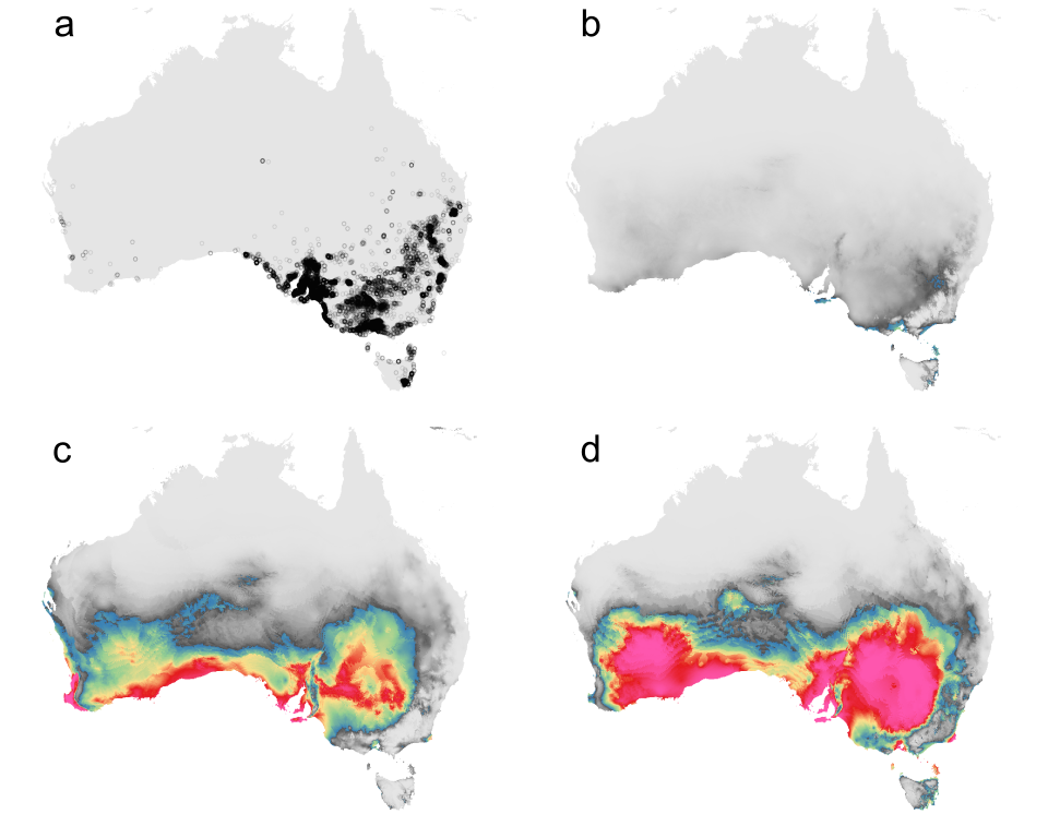
Figure 7.6 Maxent projection of climate suitability in Australia for the southern African species Lycium ferrocissimum. (a) Australian distribution according to GBIF .https://doi.org/10.15468/dl.v68j87; (b) projection using four best PCA variables, (c) using the default 19 bioclimatic variables and (d) using only five bioclimatic variables justified upon examination of climate covariance. Southern African occurrence data for model training were obtained from GBIF (https://doi.org/10.15468/dl.nf2w3y) and subjected to minor cleaning only. Models produced qualitatively similar results when projected into South Africa, but not when extrapolated to Australia.

Having used the model to create a set of outputs, how robust and plausible are the projections? There are several methods available for quantifying model performance. Some are incorporated into SDM software packages and each has its own assumptions, attributes and sensitivities (Meyer and Pebesma 2021).

Elith and Graham (2009) recommend that multiple metrics should be used for assessing the quality of model outputs. Guisan and Zimmermann (2000) and Warren et al. (2020), however, argue that the metric should depend on the objective of the study: metrics for quantifying the fit of the model to data from within its known range (i.e. model sensitivity), for example, rarely measure the model’s ability to extrapolate or its ability to describe the niche. Even if the model outputs measure up as statistically robust, are they at all ecologically plausible? A quick scan of the plethora of modelling papers from recent years will reveal biogeographic patterns that would confound the purists. Many of these illogical projections relate to inappropriate application of the model in extrapolation space, emphasising the need to tread carefully (if at all) when going beyond what is known (Mesgaran et al. 2014).

A final issue regarding SDMs relates to the way that the results are presented. This decision is usually left to software developer defaults rather than a choice of the user. Maps of projected ‘suitability’ (or the range of other spatially displayed metrics that models produce) are an essential component of the interpretation and communication of SDM results. Even if we use mathematical methods to calculate the levels of error, decisions on whether to accept a projection are heavily influenced by the visual cues: does the map look sensible? We assume that the map conveys a reliable interpretation of the SDM’s output.

Most attributes of map design are arbitrary, but it would be a mistake to dismiss them as irrelevant (Douglass and Fish 2022). Research on data visualisation shows that the choice of colours, the steepness of the colour gradient and the number of colour categories can influence the perception of information by the reader (Crameri et al. 2020). The output from an SDM is usually an index on a continuous scale and the cut-off value, for a location to be regarded as suitable to the species, can be subjective. The steepness of the colour gradient could influence decisions about the extent of relative suitability, especially where there are no occurrence observations to use for validation (such as projections into changed climates or introductions into new regions). Pixel size is also likely to be influential: a map showing the output from a poorly parameterised SDM using small pixels (i.e. an apparently high spatial precision of the input data) may easily be construed as being more trustworthy (higher quality output) than a more ecologically plausible SDM projection presented with larger pixels, simply because of its grain. Again, the risk of conflating resolution with realism is high. In any case, the SDM itself is only a hypothesised distribution; one of the most common mistakes is to treat this hypothesis as a project endpoint rather as a precursor of future research.

7.5.4 Peer review

Species distribution models continue to be developed, incorporating more biologically based mechanistic approaches (Schouten et al., 2020) and being linked to demographic and dispersal models. They are undoubtedly a useful technique if applied to the right question, parameterised appropriately and interpreted conservatively. It is easy, however, with minimal familiarisation or basic training, to produce visually appealing output from an SDM. Within a short period, anyone can download data from an online records database, run an off-the-shelf SDM using default values and put the results into a paper that is accepted by reviewers and editors with no more training than the author.

Indeed, automated software with next to no warning messages has been created to deliver this exact output. We deliberately do not include examples here to discourage the use of these highly automated packages. When these results are published in a scientific journal, readers almost invariably make the assumption that what they read is trustworthy, since the paper has been through peer review. Yet our quality control systems in science rely on a high degree of trust in the author that they are proficient in the methods they apply and that the review process will filter out sub-standard work.

Yackulic et al. (2013), however, found that 87% of articles using Maxent were based on data that were likely to suffer from sample selection bias, 36% arbitrarily discarded absence data in order to use that model and 54% incorrectly interpreted the output as occurrence probability. Kriticos et al. (2013) also listed several common problems:

• inappropriate model application;

• incorrect attribution of causality to model extrapolation artefacts;

• oversight of significant, inconvenient methodological caveats;

• extrapolation without identifying the extrapolation space; and

• failing to reconcile models with ecological theory.

The issues had clearly been missed, or regarded as unimportant, by the researchers, the reviewers and the editors!

With so many researchers publishing SDM work, it is increasingly challenging to identify reviewers who are competent enough to detect shortcomings in the deluge of SDM manuscripts that are submitted to journals each week. It may be that, in many cases, these issues had little impact on the model outputs, but most readers are not provided with the material to make this assessment. A related issue is that bad practices can snowball. While reviewing papers, the authors of this chapter have seen severely flawed modelling approaches being defended by virtue of already having been published elsewhere.

As editors and referees, we have seen examples of papers that we have recommended to be rejected (with justification), published at a later stage in other journals with few (if any) additional changes. Given how hard it can be to confidently interpret SDM outputs, there would be a strong case for deciding against publishing at all, even for carefully parameterised models. However, the pressure to publish means that rarely would a researcher get to the end of a modelling activity and decide that the outputs are not of a high enough standard to take on into the publication process.

How, then, are non-specialist readers to judge whether the authors of a given paper have chosen an appropriate model, adequately considered the properties of the data and the assumptions of the methods and taken all these things into account when considering their results? Clearly this judgement is impossible!

We know that all models are wrong (Box 1979), but maybe it is impossible for non-specialist readers to know which are useful. In response to the documented high incidence of problems, only one journal seems to have formally adopted a reporting protocol published by concerned authors (for which an app is also available; Zurell et al. 2020). Why have more editorial boards not taken action when they are alerted to widespread misuse of methods? Even if they did, who would decide on what falls on the right side of the line when it comes to methodological options for a given context? If there’s one thing that we all know, ecologists are known to regularly and robustly disagree. Creating further inertia, the incredible citation rates of SDM papers and the relative ease by which they can be generated is a powerful drug to give up in an industry where employment opportunities and career progressions remain heavily influenced by publication metrics.

It can be argued that, ultimately, it is the responsibility of the users of SDMs to make sure that they are adequately trained. Such training is now more widely available than it was perhaps a decade ago, but there is little evidence to suggest that it is being taken up or that the recommendations are being implemented. Crucially, we must also remember that the models we produce are not endpoints of research, but instead are hypotheses to be tested.

To do better, we need to inform users not just about what they need to do, but what they should not do. When should a modelling venture be abandoned due to inadequate data or poor model performance? How are SDM practitioners to know when their knowledge is sufficiently adequate? Warnings by expert practitioners and model developers do not appear to reach the attention of occasional users (Yackulic et al. 2013; Morales et al. 2017), especially now that most scientists do not browse journal contents. Likewise, reviewers and editors may not know what to look for. Our peer review system would grind to a halt if we insisted that every piece of work be adjudicated on by an expert in every technique used in a study.

7.6 So what?

Ecology would not be possible without assumptions. Assumptions are indispensable to scientists, because they help us to cope with the complicated world that we are trying to interpret. We must embrace them and respect them, because they are at the heart of what we can and cannot claim to have discovered in our research. If our assumptions are inappropriate or incorrect, then we can make serious errors in our conclusions. It is therefore essential for us to develop a robust knowledge of what they are, the context in which they are relevant, the extent to which they matter and what we can do to make sure that we are not misled. To proceed in research as if the plausibility of our assumptions does not matter would surely be unwise.

Some of the assumptions that we make in ecology may be impossible to test, or at least it would require major additional investigation to do so. This challenge is a common reason why assumptions are required! For example, testing the extent to which individuals within a study area undergo random mating or whether immigration and emigration balance one another would require unjustified effort for most studies. We rely on any departure from the assumption being either unimportant or acting equally across all situations that we are comparing, so that it is relatively unimportant. Without making assumptions, it might be difficult to make progress.

In some situations we may use an assumption without even expecting it to be valid, but we use it as a way to better understand our study system. There are many examples where we use a theoretical model to tell us what we would expect – a null prediction – and then see how far our data depart from that prediction. But there are also a great many situations in which departures from our assumptions can seriously affect the interpretations of our data and, in turn, the entire findings of our research. A good example of this is analysis of variance.

In this chapter, we highlighted the many assumptions that, if they are not fulfilled by our data, have the potential to undermine or invalidate conclusions about invasion niche shifts and species distribution outputs. It would be self-deluding for us to make the bold additional assumption that, in any given study, inappropriate assumptions either do not occur or that they do not matter, if we have not made the effort to test their validity and communicate this effectively in our reporting. There is considerable evidence, particularly from the descriptions of data analysis, that many researchers do not follow good practice for checking assumptions and that unsafe conclusions may, as a result, easily be reached. Readers and end-users of this research could also potentially be misled – especially if they are not themselves experts in the methods that have been used and who accept our conclusions at face value (Box 7.2).

A discussion with an expert in almost any ecological method will often reveal that examples of poor practice are frequent. Faced with this, our advice to any reader of a paper, at least initially, is to be sceptical of every paper that they read unless the author explicitly states what the assumptions were, how they checked them and whether they considered them influential on the findings. We encourage the future leaders of ecological research to hone their skills by probing these papers further: identifying assumptions that remain implicit, probing for those that could undermine the findings and seeking out exemplar papers that lead the way in best practice research methods. Is it time for the recent progress we have seen in the open data movement (Wessels et al. 2017) to motivate equivalent momentum in open, transparent and accountable research as it applies to assumptions?

In empirical research, such as the analysis of species ranges that we used here as a case study, ecologists frequently try to extract as much as they can – no matter how inadequate the data – and to see how much support there is for an established idea or concept. The research becomes driven by the data that we currently have, rather than what we would need to have in order to achieve a particular objective. The more assumptions that we have to make about our data and our methods, and the weaker the support for those assumptions, then the less confident we should be in our assertions. Meta-analyses of many weak studies should not be interpreted as strong support for a particular conclusion, since all the studies may have the same weak underlying assumptions. We should beware of strong assertions of fact in banner headlines of papers.

As we discussed in the case of species distribution models, lack of attention to assumptions in ecological research is often not picked up in the peer review process. In our experience (and in discussions with other editors), it would appear to be rare for the editor-in-charge of a journal to communicate about topical problems – such as the recently and widely reported frequent misuses of SDMs – with their associate editors or to announce a policy for addressing the issue. Some journals publish, and perhaps even seek out, articles for their journal on a topic of particular concern. We assume – falsely – that these papers will be widely read and that their recommendations will be adopted.

Only one journal, to our knowledge, has adopted a code of practice for SDMs. When we asked a senior editor of a major ecological journal why actions have not been taken by that journal to address the widespread publication of misuse of SDMs, they pointed out that SDMs are only one of many methodological problems in the ecological literature and it is impossible to seek to overcome them all. This is almost certainly true, but it is surely also a disturbing report. We are cognisant of the fact that a great deal is expected of our journal editors and reviewers. But while the responsibility for good ecological practice may ultimately be with the researcher, the discipline as a whole would benefit from more comprehensive efforts to clean up particular bad practices.

At what point is the lack of congruence between data and assumptions a problem? Does it matter enough for us to either dismiss our study or to take some form of remedial action? There are objective criteria for some methods, which we can report on in a paper’s supplementary information in order to satisfy others. But often the decision is a subjective one, requiring experience and judgement. Many users of ecological methods, however, are yet to develop sufficient expertise. It is not surprising if there is some element of ‘hoping for the best’. It is worth noting here that, increasingly, we use readily available, user-friendly software or someone else’s code to analyse data. Just because we can process data efficiently does not mean that it provides a quality control mechanism for the user: it simply means that it is easy to produce output. The capacity to check for the acceptability of assumptions is usually available, but often as an option and not as a default.

If the user does not appreciate the need to check particular assumptions, then they cannot be expected to do so. It could be argued that software developers should be responsible for including routine checks into their programs, even at the risk that these will antagonise experienced researchers. Yet native scripting (e.g. in R or Python) is fast coming to dominate ecological analyses and the variability in associated documentation is considerable. Once again, we see the onus on ensuring best practice methods, including giving consideration to any assumptions, falling back to the user (and in turn those who educate new users).

We are in danger of losing our science down a rabbit hole of unfounded assumptions, bewildering methodologies and untested hypotheses.

Facing this precipice, we might feign ignorance, inattentively copying whatever has been done in the past. After all, advancement in academia is increasingly difficult, and researchers worldwide have increasingly less time to devote to contemplative thought and pushing back on convention. Or perhaps we should throw up our hands in disgust and abandon the effort entirely – as the authors of this chapter are often tempted to do with SDMs! Alluring as these options may be, the fact remains that complex ecological methodologies are here to stay with their layers of underpinning assumptions, and are needed to protect biodiversity, natural resources and human health in an era of rapid global change.

As daunting as it may seem, we encourage you (our ecologist superstars of the future) to warmly embrace assumptions for what they are. We must, as a research discipline, get better at keeping track of our assumptions as they accumulate in computational, conceptual or statistical models, and give explicit consideration to how those assumptions influence our inferential power. It should become de rigueur to weigh the ‘assumption cost’ of the decisions we make and to share our concerns, caveats and limitations with our readers in an open and accountable way.

We also need brave, clear-headed scientists who can cut through the noise, critically evaluate our assumptions and chart a path forward. This is true not just for the examples we have used in this chapter, but for all of ecology, which is reckoning with the need to anticipate the future in an increasingly confusing and volatile landscape (Maris et al. 2018).

We hope that readers of this chapter will approach their own research and reading with a renewed sense of both scepticism and of the importance and power of assumptions. If we treat an assumption not as a thing to be ignored or evaded but as a tool to be wielded, we may need to limit our scope of inference, but our predictions and projections will be more focused and powerful. Time will tell what role our currently applied ecological methods will play in the future of ecology, but whatever value they have will be maximised only if we treat our assumptions with the respect that they deserve. Our science is, after all, only as good as our assumptions.

7.7 References

Atwater, D. Z., C. Ervine, and J. N. Barney. 2018. Climatic niche shifts are common in introduced plants. Nature Ecology and Evolution 2:34–43. doi:10.1038/s41559-017-0396-z

Baker, H. G., and G. L. Stebbins (eds). 1965. The genetics of colonizing species. New York: Academic Press.

Begon, M., J. L. Harper, and C. R. Townsend. 1996. Ecology, 3rd edition. Oxford: Blackwell Science.

Booth, T. H., H. A. Nix, J. R. Busby, and M. F. Hutchinson. 2014. BIOCLIM: the first species distribution modelling package, its early applications and relevance to most current MaxEnt studies. Diversity and Distributions 20:1-9. doi:10.1111/ddi.12144

Box, G. E. P. 1979. Robustness in the strategy of scientific model building. In Robustness in statistics, eds Launer, R. L. and G. N. Wilkinson Academic Press, 201–236. doi:10.1016/B978-0-12-438150-6.50018-2

Cousens, R. 1988. Misinterpretations of results in weed research through inappropriate use of statistics. Weed Research 28:281 289.

Cousens, R. D., P. K. Ades, M. B. Mesgaran, and S. Ohadi. 2013. Reassessment of the invasion history of two species of Cakile (Brassicaceae) in Australia. Cunninghamia 13:275-290. doi:10.7751/cunninghamia.2013.005

Crameri, F., G. E. Shephard, and P. J. Heron. 2020. The misuse of colour in science communication. Nature Communications 11:5444. doi:10.1038/s41467-020-19160-7

Daly, C. 2006. Guidelines for assessing the suitability of spatial climate data sets. International Journal of Climatology 26:707–721. doi:10.1002/joc.1322

Davis, A.J., L. S. Jenkinson, J. H. Lawton, et al. 1998. Making mistakes when predicting shifts in species range in response to global warming. Nature 391:783–786. doi:10.1038/35842

Dormann, C.F., O. Purschke, J. R. García Márquez, et al. 2008. Components of uncertainty in species distribution analysis: A case study of the great grey shrike. Ecology 89:3371-3386. doi:10.1890/07-1772.1

Douglass, N. A. K., and C. S. Fish. 2022. That’s a relief: assessing beauty, realism, and landform clarity in multilayer terrain maps. Cartographic Perspectives 100:45-66. doi:10.14714/CP100.1727

Elith J., M. Kearney, and S. Phillips. 2010. The art of modelling range‐shifting species. Methods in Ecology and Evolution 1:330-342. doi:10.1111/j.2041-210X.2010.00036.x

Elith, J. 2017. Predicting distributions of invasive species. In Invasive Species: Risk assessment and management, eds T.R. Walshe, A. Robinson, M. Nunn and M.A. Burgman, 93-129. Cambridge: Cambridge University Press. doi:10.1017/9781139019606

Elith, J., and C. H. Graham. 2009. Do they? How do they? WHY do they differ? On finding reasons for differing performances of species distribution models. Ecography 32:66-77. doi:10.1111/j.1600-0587.2008.05505.x

Elith, J., and J. Franklin. 2013. Species Distribution Modeling. In Encyclopedia of Biodiversity: Second Edition, ed. S. M Scheiner, 692-705. San Diego: Elsevier.

Elith, J., C. H. Graham, R. P. Anderson, et al. 2006. Novel methods improve prediction of species’ distributions from occurrence data. Ecography 29:129-151. doi:10.1111/j.2006.0906-7590.04596.x

Elith, J., S. J. Phillips, T. Hastie, et al. 2011. A statistical explanation of MaxEnt for Ecologists. Diversity and Distributions 17:43–57. doi:10.1111/j.1472-4642.2010.00725.x

Ellenberg, H. 1974. Zeigerwerte der Gefässpflanzen Mitteleuropas. Scripta Geobot Göttingen 9:1-97.

Fick, S.E., and R. J. Hijmans. 2017. WorldClim 2: New 1-km spatial resolution climate surfaces for global land areas. International Journal of Climatology 37:4302-4315. doi:10.1002/joc.5086

Fitzpatrick, M.C., and W. W. Hargrove. 2009. The projection of species distribution models and the problem of non-analog climate. Biodiversity and Conservation 18:2255–2261. doi:10.1007/s10531-009-9584-8

Forcella, F. 1985. Final distribution is related to rate of spread in alien weeds. Weed Research 25:181-191. doi:10.1111/j.1365-3180.1985.tb00634.x

Fréjaville, T., and M. B. Garzón. 2018. The EuMedClim database: Yearly climate data (1901–2014) of 1 km resolution grids for Europe and the Mediterranean basin. Frontiers in Ecology and Evolution 6:31. doi:10.3389/fevo.2018.00031

Grinnell, J. 1917. The niche-relationships of the California Thrasher. The Auk 34:427-433.

Guisan, A., and N. E. Zimmermann. 2000. Predictive habitat distribution models in ecology. Ecological Modelling 135:147-186. doi:10.1016/S0304-3800(00)00354-9

Guisan, A., and W. Thuiller. 2005. Predicting species distribution: offering more than simple habitat models. Ecology Letters 8:993–1009. doi:10.1111/j.1461-0248.2005.00792.x

Guisan, A., B. Petitpierre, O. Broennimann, et al. 2014. Unifying niche shift studies: insights from biological invasions. Trends in Ecology and Evolution 29:260-269. doi:10.1016/j.tree.2014.02.009

Hallgren, W., F. Santana, S. Low-Choy, et al. 2019. Species distribution models can be highly sensitive to algorithm configuration. Ecological Modelling 408:1-23. doi:10.1016/j.ecolmodel.2019.108719

Hao, T., J. Elith, G. Guillera-Arroita, and J. J. Lahoz-Monfort. 2019. A review of evidence about use and performance of species distribution modelling ensembles like BIOMOD. Diversity and Distributions 25:839-852. doi:10.1111/ddi.12892

Hargreaves, A.L., K. E. Samis, and C. G. Eckert. 2014. Are species’ range limits simply niche limits writ large? A review of transplant experiments beyond the range. The American Naturalist 183:157-173. doi:10.1086/674525

Holt, R. D. 2009. Bringing the Hutchinsonian niche into the 21st century: Ecological and evolutionary perspectives. Proceedings of the National Academy of Sciences of the United States of America 116 (Suppl. 2):19659-19665. doi:10.1073/pnas.0905137106

Hutchinson, G. E. 1978. An introduction to population ecology. New Haven: Yale University Press.

Jackson, S. T., and J. T. Overpeck. 2000. Responses of plant populations and communities to environmental changes of the late Quaternary. Paleobiology 26:194-220.

Keane, R. M., and M. J. Crawley 2002. Exotic plant invasions and the enemy release hypothesis. Trends in Ecology and Evolution 17:164-170. doi:10.1016/S0169-5347(02)02499-0

Kearney, M.R., and W. P. Porter. 2020. NicheMapR – an R package for biophysical modelling: the ectotherm and Dynamic Energy Budget models. Ecography 43:85-96. doi:10.1111/ecog.04680

Keyfitz, N. 1972. On future population. Journal of the American Statistical Association 67:347-363.

Kriticos, D. J., B. L. Webber, A. Leriche, et al. 2012. CliMond: global high-resolution historical and future scenario climate surfaces for bioclimatic modelling. Methods in Ecology and Evolution 3:53-64. doi:10.1111/j.2041-210X.2011.00134.x

Kriticos, D. J., D. C. Le Maitre, and B. L. Webber. 2013. Essential elements of discourse for advancing the modelling of species’ current and potential distributions. Journal of Biogeography 40:608–613. doi:10.1111/j.1365-2699.2012.02791.x

Kriticos, D. J., L. Morin, and B. L. Webber. 2014. Taxonomic uncertainty in pest risks or modelling artefacts? Implications for biosecurity policy and practice. NeoBiota 23:81-93. doi:10.3897/neobiota.22.7496

Lande, R. 2014. Evolution of phenotypic plasticity and environmental tolerance of a labile quantitative character in a fluctuating environment. Journal of Evolutionary Biology 27:866–875. doi:10.1111/jeb.12360

Liu, C., C. Wolter, W. Xian, and J. M. Jeschke. 2020. Most invasive species largely conserve their climatic niche. Proceedings of the National Academy of Sciences of the United States of America 117:23643–23651. doi:10.1073/pnas.2004289117

Lowry, E., E. J. Rollinson, A. J. Laybourn, et al. 2013. Biological invasions: a field synopsis, systematic review, and database of the literature. Ecology and Evolution 3:182–196. doi:10.1002/ece3.431

Maycock, C.R., E. Khoo, C. J. Kettle, et al. 2012. Using high resolution ecological niche models to assess the conservation status of Dipterocarpus lamellatus and Dipterocarpus ochraceus in Sabah, Malaysia. Journal of Forest and Environmental Science 28:158-169. doi:10.7747/JFS.2012.28.3.158

Merow, C., M. J. Smith, and J. A. Silander. 2013. A practical guide to MaxEnt for modeling species’ distributions: what it does, and why inputs and settings matter. Ecography 36:1058-1069. doi:10.1111/j.1600-0587.2013.07872.x

Mesgaran, M. B., R. D. Cousens, and B. L. Webber. 2014. Here be dragons: a tool for quantifying novelty due to covariate range and correlation change when projecting species distribution models. Diversity and Distributions 20:1147–1159. doi:10.1111/ddi.12209

Meyer, C., P. Wiegelt, and H. Kreft. 2016. Multidimensional biases, gaps and uncertainties in global plant occurrence information. Ecology Letters 19:992-1006. doi:10.1111/ele.12624

Meyer, H., and E. Pebesma. 2021. Predicting into unknown space? Estimating the area of applicability of spatial prediction models. Methods in Ecology and Evolution 12:1620-1633. doi:10.1111/2041-210X.13650

Morales, N. S., I. C. Fernández, and V. Baca-González. 2017. MaxEnt’s parameter configuration and small samples: are we paying attention to recommendations? A systematic review. PeerJ 5:e3093. doi:10.7717/peerj.3093

Newbold, T., T. Reader, A. El-Gabbas, et al. 2010. Testing the accuracy of species distribution models using species records from a new field survey. Oikos 119:1326-1334. doi:10.1111/j.1600-0706.2009.18295.x

Noce, S., L. Caporaso, and M. Santini. 2020. A new global dataset of bioclimatic indicators. Scientific Data 7:398. doi:10.1038/s41597-020-00726-5

Peterson, A. T., and J. Soberón. 2012. Integrating fundamental concepts of ecology, biogeography, and sampling into effective ecological niche modeling and species distribution modeling. Plant Biosystems 146:789-796. doi:10.1080/11263504.2012.740083

Petitpierre, B., C. Kueffer, O. Broennimann, et al. 2012. Climatic niche shifts are rare among terrestrial plant invaders. Science 335:1344-1348. doi:10.1126/science.12159

Phillips, S. J., R. P. Anderson, M. Dudík, et al. 2017. Opening the black box: an open‐source release of Maxent. Ecography 40:887-893. doi:10.1111/ecog.03049

Phillips, S.J., M. Dudík, J. Elith, et al. (2009). Sample selection bias and presence-only distribution models: implications for background and pseudo-absence data. Ecological Applications 19:181–197. doi:10.1890/07-2153.1

Pyron, R. A., G. C. Costa, M. A. Patten, and F. T. Burbrink. 2015. Phylogenetic niche conservatism and the evolutionary basis of ecological speciation. Biological Reviews 90:1248-1262. doi:10.1111/brv.12154

Ratcliffe, S. ed. (2017) Oxford essential quotations, 5th edn. Oxford: Oxford University Press.

Roughgarden, J. 1974. Niche width: Biogeographic patterns among Anolis lizard populations. The American Naturalist 108:429-442. doi:10.1086/282924

Royle, J. A., R. B. Chandler, C. Yackulic, and J. D. Nichols. 2012. Likelihood analysis of species occurrence probability from presence-only data for modelling species distributions. Methods in Ecology and Evolution 3:545–554. doi:10.1111/j.2041-210X.2011.00182.x

Schoener, T. W. 1968. Anolis lizards of Bimini: resource partitioning in a complex fauna. Ecology 49:704–726. doi:10.2307/1935534

Schouten, R., P. A. Vesk, and M. R. Kearney. 2020. Integrating dynamic plant growth models and microclimates for species distribution modelling. Ecological Modelling 435:109262. doi:10.32942/osf.io/ja4m6

Schröter, M., Crouzat, E., Hölting, L. et al. 2021. Assumptions in ecosystem service assessments: Increasing transparency for conservation. Ambio 50:289–300. doi:10.1007/s13280-020-01379-9

Sutherst, R. W. 2003. Prediction of species geographical ranges. Journal of Biogeography 30:805-816.

Syfert, M. M., M. J. Smith, and D. A. Coomes. 2013. The effects of sampling bias and model complexity on the predictive performance of MaxEnt species distribution models. PLoS ONE 8:e55158. doi:10.1371/journal.pone.0055158

Thuiller, W., B. Lafourcade, R. Engler, and M. B. Araújo et al. 2009. BIOMOD – A platform for ensemble forecasting of species distributions. Ecography 32:369-373. doi:10.1111/j.1600-0587.2008.05742.x

Tyberghein, L., H. Verbruggen, K. Pauly, et al. 2011. Bio-ORACLE: a global environmental dataset for marine species distribution modelling. Global Ecology and Biogeography 21:272-281. doi:10.1111/j.1466-8238.2011.00656.x

van Boheemen, L. A., D. Z. Atwater, and K. A. Hodgins. 2019. Rapid and repeated local adaptation to climate in an invasive plant. New Phytologist 222:614–627. doi:10.1111/nph.15564

van Proosdij, A. S. J., M. S. M. Sosef, J. J. Wieringa, and N. Raes. 2016. Minimum required number of specimen records to develop accurate species distribution models. Ecography 39:542-552. doi:10.1111/ecog.01509

Warren, D. L., N. J. Matzke, and T. L. Iglesias. 2020. Evaluating presence-only species distribution models with discrimination accuracy is uninformative for many applications. Journal of Biogeography 47:1670-180. doi:10.1111/jbi.13705

Webber, B. L., C. Born, B. J. Conn, et al. 2011a. What is in a name? That which we call Cecropia peltata by any other name would be as invasive? Plant Ecology and Diversity 4:289-293. doi:10.1080/17550874.2011.610372

Webber, B. L., C. J. Yates, D. C. Le Maitre, et al. 2011b. Modelling horses for novel climate courses: insights from projecting potential distributions of native and alien Australian acacias with correlative and mechanistic models. Diversity and Distributions 17:978-1000. doi:10.1111/j.1472-4642.2011.00811.x

Webber, B. L., D. C. Le Maitre, and D. J. Kriticos. 2012. Comment on ‘Climatic niche shifts are rare among terrestrial plant invaders’. Science 338:193. doi:10.1126/science.12259

Wessels, B., R. Finn, T. Sveinsdottir, and K. Wadhwa eds. 2017. Open data and the knowledge society. Amsterdam: Amsterdam University Press.

Wiens, J. A., D. Stralberg, D. Jongsomjit, et al. 2009. Niches, models, and climate change: Assessing the assumptions and uncertainties. Proceedings of the National Academy of Sciences of the United States of America 106 (Suppl. 2):19729-19736. doi:10.1073/pnas.0901639106

Wisz, M. S., R. J. Hijmans, J. Li, A. T. Peterson, et al. 2008. Effects of sample size on the performance of species distribution models. Diversity and Distributions 14:763–773. doi:10.1111/j.1472-4642.2008.00482.x

Xu S., J. Wang, Z. Guo et al. 2020. Genomic convergence in the adaptation to extreme environments. Plant Communications 1:100117. doi:10.1016/j.xplc.2020.100117

Yackulic, C. B., R. Chandler, E. F. Zipkin, et al. 2013. Presence-only modelling using MAXENT: When can we trust the inferences? Methods in Ecology and Evolution 4:236-243. doi:10.1111/2041-210x.12004

Zizka, A., D. Silvestro, T. Andermann, et al. 2019. CoordinateCleaner: Standardized cleaning of occurrence records from biological collection databases. Methods in Ecology and Evolution 10:744-751. doi:10.1111/2041-210X.13152

Zurell, D., J. Elith, and B. Schröder, B. 2012. Predicting to new environments: tools for visualizing model behaviour and impacts on mapped distributions. Diversity and Distributions 18:628–634. doi:10.1111/j.1472-4642.2012.00887.x

Zurell, D., J. Franklin, C. König, et al. 2020. A standard protocol for reporting species distribution models. Ecography: 43:1261-1277. doi:10.1111/ecog.04960