Chapter 7 The Open Economy
At the end of this chapter you should understand the following:
The open economy extension of the New Keynesian model
Uncovered Interest Parity (UIP)
The medium run AD-ERU model
Central bank stabilisation in the open economy
Opening the economy to the rest of the world means that there are other countries buying and selling goods and services and foreign exchange traders trying to anticipate exchange rates and interest rates. There is interaction with the rest of the world. The central bank must try to estimate the effect of exchange rates on the economy. Interest rates and exchange rates affect the economy with a lag of one period. International investors will take advantage of different rates of return to move money to currencies that have the highest return.
7.1 Foreign exchange
We assume that the nominal exchange rate \((e)\) is the domestic currency that can be bought with one unit of foreign currency. In some places you will see rates quoted the other way around. This means that the exchange rate appreciates when it goes down (as it becomes more valuable and you give less of it away to get foreign currency).
\[e = \frac{\text{domestic currency}}{\text{foreign currency}}\]
A rise in e is a depreciation of the domestic currency.
The real exchange rate is defined as
\[Q = \frac{\text{price of foreign goods in home currency}i}{\text{price of home goods}} = \frac{P^*e}{P}\]
Where \(P\) is the price level, \(P^*\) is the overseas price level and \(Q\) is a measure of competitiveness. A rise in \(Q\) means that domestic goods are becoming cheaper. An increase in \(Q\) will increase net exports (real exports less real imports) and affect aggregate demand through net exports. Now there is a second channel through which interest rates affect the economy: if inflation is above target, the central bank will raise interest rates to bring the economy below its potential and to put downward pressure on inflation; the foreign exchange market will anticipate this and will purchase GBP at the expense of USD, thereby driving up the value of the pound (e falls and, depending on \(P\) and \(P^*\), \(Q\) also falls), reducing competitiveness and net exports and adding to the interest rate effect on aggregate demand. The adjustment is shared by interest rates and the exchange rate. This is based on the assumption that the central bank and actors in the foreign exchange market work on the basis of rational expectations. This is more dubious for the foreign exchange market than it is for the central bank. We know that financial markets can be driven by manias and by herding. However, this can be the staring point to get the baseline idea.
7.2 The New Keynesian model.
For the open economy, the IS curve must be amended to include net exports. The multiplier will be less powerful here because some of the increase in demand will leak abroad. The IS curve will become steeper because a given change in interest rates will have a smaller effect on aggregate output. A change in competitiveness will shift the IS curve inwards or outwards. The Phillips curve does not change much. We continue to work on the assumption that there is a unique level of unemployment for stabilisation and that this is determined by the WS curve (based on supply side changes in the cost of job loss, wage bargaining arrangements and employment regulations etc) and the PS curve (based on changes in the level of competition, the tax wedge etc). The MR function will continue to be based on the loss function that comes from unemployment and inflation. In this case we will look at domestic inflation rather than that imported from abroad. Global capital flows are now important: the foreign exchange market has an influence on aggregate demand and households are able to purchase domestic and foreign assets. In a world without international capital flows, the price of foreign exchange is determined by the supply and demand for goods. However, as capital flows become more important, these capital flows become a more significant influence on exchange rates.
There are a number of simplifications that will be made. Firstly, we will assume that the bond market represents a range of different asset markets. There are just two assets that can be purchased: bonds or money. There is perfect international capital mobility. This means that domestic agents can buy and sell unlimited quantities of domestic and overseas assets with low transaction costs. The home country is small and it is assumed that it does not affect the world interest rate. There is perfect substitutability of domestic and foreign bonds. This means that the risk is the same and the only question is the rate of return. The final assumption is one that may or may not hold. See discussion of the Eurozone for more on this.
The expected return on bonds is a function of the return on the bond and the exchange rate. The interest rate set by the central bank and the return on the bond are related because they are substitutes. The exchange rate return is based on uncovered interest parity (UIP). It is assumed that exchange rate forecasts are based on (rational expectations. This is a contrast to the inflation forecasts which are made on adaptive expectations. The difference is justified by saying that households use professional agents to make investment decision on their behalf while forming expectations about inflation themselves. Figure 9.1 shows the adjustment of interest rates and exchange rate to maintain returns.
Uncovered Interest Parity (Carlin and Soskice 2015)
7.3 Modelling
UIP is based on
\[i - i^* = \frac{e^E_{t+1} - e_t}{e_t}\]
A change in interest rates will affect the current exchange rate. The expected exchange rate is not changed. This will be modelled later. Using a log approximation,
\[\frac{e^E_{t+1} - e_t}{e_t} = ln e_{t+1}^E - ln e_t \]
Therefore,
\[i^* - i =\frac{e^E_{t+1} - e_t}{e_t} \]
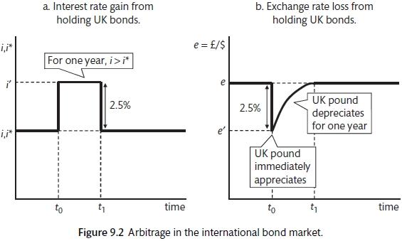
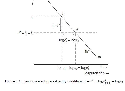
The interest rate differential equals the change in the exchange rate. Figure 9.2 shows the relationship between the exchange rate and the domestic interest rate when the world interest rate is pinned down to an exogenous level. The model can also be used to look at the effect of a change in world interest rates. This will result in a parallel shift in the 45 degree line. It will change the domestic interest rate that is associated with the stable exchange rate. The model can also be used for modelling expectations about changes in the future exchange rate. This will also result in a shift in the UIP curve.
The world interest rate and the exchange rate (Carlin and Soskice 2015)
7.4 Medium-term equilibrium
The medium-term equilibrium is when inflation is constant. This depends on equilibrium in the labour market when the WS and PS curves intersect. This will pin down the Equilibrium Rate of Unemployment (ERU). Leaving trade aside for now, the ERU represents supply in the exchange rate-output space. The Aggregate Demand curve (AD) shows equilibrium in the goods market when the interest rate is at the level of the **world interest rate (r^*)**. Figure 9.3 brings together the labour market (through ERU) and AD. Though not shown here, the short-run Phillps Curves (PC) are derived in the same was as in the closed economy. The log of the real exchange rate is used here (q). The ERU curve can be defined as
\[y - y_e(Z^W, Z^P)\]
with \(Z^W\) factors that affect the wage setting curve (unionisation, regulation and benefits) and \(Z^P\) factors that affect price setting (level of competition, tax and technology).
AD incorporates demand and the UIP condition. This is a version of the IS curve with a positive adjustment to lower interest rates (with a one period lag) and a positive adjustment to an depreciation of the exchange rate (with a one period lag).
\[y_t = A_t - ai_{t-} + bq_{t-1}\]
This is the open-economy IS curve, where A includes the multiplier and demand shift variables such as world trade, government spending and factors that shift consumption and investment such as wealth and Tobin’s Q. In the medium term the exchange rate is equal to its equilibrium expected value. If the UIP condition is
\[i_t - i^*_t = log e^E_{t+1} - log e_t\]
The real UIP is
\[r_t - r_t^* - q^E_{t+1} - q_t\]
r = r^ * in the medium term to ensure that the exchange rate is stable. Therefore, the medium term IS becomes
\[y = A - ai^* + bq\]
the AD curve is sloping upwards in the real exchange rate - output space as the more depreciation the more output.
The medium term analysis for a small open economy relies on the AD demand (which shows the equilibrium when \(r = r^*\)), the supply equilibrium with the ERU and the interest rate of the AD and ERU where the real exchange rate is equal to its medium term value, output is at the rate that keep inflation constant and the interest rate is at the level of the world interest rate.
7.5 Medium run real exchange rate
In this model the real interest rates is pinned down by the world interest rate and therefore it is the exchange rate that must adjust to supply and demand shocks. For example, if there is a positive productivity shock, this will shift the PS curve upwards, moving the ERU to the right. At the higher level of output, there must be a depreciation of the real exchange rate to encourage output to the higher level. On the other side, a positive investment shock will shift the AD curve to the left and this will mean that the real exchange rate must appreciate to choke off demand in other areas so that overall output remains unchanged.
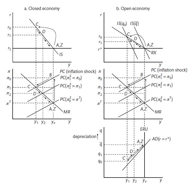
For medium-term stabilisation policy the AD-ERU model is used with the addition of the RX curve that gives the central bank policy response taking into account the exchange rate. To simplify the modelling here it is assumed that the central bank targets domestic inflation. In reality they will target consumer inflation that also includes imported prices. In the closed economy the central bank minimises its loss function by setting interest rates, with an open economy the central bank has the same loss function but must now look at the effect of interest rates on the exchange rate when assessing the effect of its policy. The monetary policy (MR) rule remains the same but this is now implemented through the open-economy IS curve. Taking into account the effect of interest rates on the exchange rate (via UIP), the central bank will respond via a flatter RX curve.
It is possible to compare the adjustment of the open and closed economies. The response to a positive inflation shock is for the central bank to raise the interest rate so that output is below equilibrium and this forces inflation back down to the target. There is inflation persistence due to the way that household inflation expectations are modelled. The central bank uses the inflation-expectations augmented Phillips curve to set interest rates such that they bring inflation gradually back to the target. In the open economy, the central bank has to consider the effect of the interest rate on the exchange rate. It does this via the RX curve. This incorporates the effect of the higher interest rate on the interest sectors of the economy \((IS)\) but also the effect of having interest rates above the world equilibrium \((r^*)\) and the way that this will shift the IS curve. As interest rates gradually come back to the international equilibrium, the IS curve shifts back to its original position. The modelling is augmented with the real exchange rate - output space and the ERU and AD curves. The RX curve is flatter than the IS curve because the interest rate has two effects.
Comparison of open and closed economy (Carlin and Soskice 2015)
Differences between closed and open economy responses: closed economy interest rate change must be greater; the IS curve shifts in the open economy as this is a results of the effect of the real exchange rate on net exports, in the closed economy the only effect is the shift along the IS curve in response to the interest rate change; the closed economy moves along the IS curve back to equilibrium, the open economy moves back only the RX curve to equilibrium. The RX curve goes through the \(r^*\) and y-e and therefore will change if either of these change. The excel model shows the impulse response functions to a change in variables.