Chapter 8 Open Supply and Demand
By the end of this chapter you should understand:
the nature of the demand side in the open economy
The concepts of the trade balance and the way that is reflected in the BT curve
The derivation and use of the downward sloping ERU curve
Analysing shocks in the AD-ERU medium-run framework
Opening the economy to the rest of the world can be useful for analysing some problems. This will depend on the question and the country. Different countries have different levels of openness. Trade openness is measured as the sum of exports and imports relative to GDP. UK openness remained stable at about 40% of GDP since the 1970s. The US has risen from about 20% in the 1980s to just less than 30% now. However, China and Germany have openness of about 60% and 70% respectively. Financial globalisation is measured as gross external assets plus liabilities as a percentage of GDP. The Balance of Payments measures the transactions between the home country and those abroad. The BOP is made up of the trade balance, the current account, the capital and financial accounts.
Trade is \(BT = X - M\). Current is trade plus net interest and profit receipts. It is useful to separate the private and public parts of the financial account.
\[BP = (BT + INT) + (F - \Delta R) = 0\]
Where INT is net factor income from abroad; \(\Delta R\) is the change in reserves. The exchange rate can be either fixed or floating. If it is fixed, the change in reserves reflect the imbalance; if it is floating, there is no change in reserves. The trade position will reflect investment and savings decisions.
Factors that affect the international demand for goods: the relative price \((Q = \frac{P^*e}{P})\). There are two sides to exchange rate depreciation: the link to competitiveness and exports; the effect on the price of imports. The Marshall-Lerner condition says that volume effect must outweigh the terms of trade effect for an appreciation of the real exchange rate to hurt the trade balance. This will be the case when the elasticity of demand for exports and imports sum to one or more. Empirical evidence suggests that this is usually the case. Import prices may affect the supply side and wage setting. If wages respond to total prices, the ERU curve may be downward sloping. If this is the case, shifts in aggregate demand can shift the economy to a new equilibrium as an appreciation of the exchange rate will reduce prices, increasing the real wage and promoting a new WS-PS equilibrium where there is lower unemployment.
Medium run (Carlin and Soskice 2015)
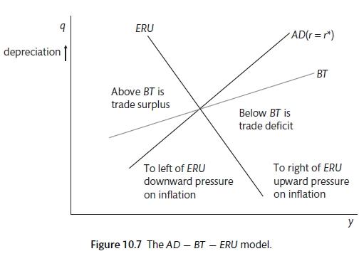
In addition to the downward sloping ERU curve it is also possible to add an upward sloping BT curve in the real-exchange rate output space. Above the BT line there is a trade surplus (with a lower real exchange rate and lower output to reduce imports) and below that there is a deficit. The BT curve will be flatter than the AD curve as the multiplier effect from the increase in output will be less strong than AD as only a proportion of the increase in output will be spent on domestic goods.
##Open economy IS curve This IS curve is steeper as the effect of the multiplier is less powerful due to some leakage abroad. The open economy IS curve will shift in response to changes in the real exchange rate \((Q)\) and to word output \((Y^*).\) The effect of a depreciation and high overseas output are not the same, a depreciation means a deterioration in the terms of trade, higher import costs and lower living standards.
Goods market is in equilibrium when output equal demand
\[y^D = c_0 + c_1(1 - t)y + I(i^*) + G + BT\]
\[BT = X - M \]
Assume to begin that exports are exogenous and imports are a fraction of output.
\[X = \bar{X}\]
\[M = my\]
\[y^D = c_0 + c_1(1 - t)y + I(i^*) + G + \bar{X} - my\]
Now solving for y
\[y = \frac{1}{1 - c_1(1 - t) + m}(c_0 + I(r) + G + \bar{X} )\]
The open economy multiplier is lower because of the marginal propensity to import (m).
8.1 Supply side and price setting
It is assumed that imperfectly competitive firms set prices on the basis of home costs using the price setting rule for the home economy. However, there are three alternative pricing methods for exports:
firms set export prices in the same way as they set home prices;
prices are set internationally.
The first is cost pricing, the second is world pricing. See how things change in different pricing regimes when there is a rise in domestic costs. In the first case, export prices rise and there is a fall in competitiveness (Q rises as P rises). In the second case, there is no loss of competitiveness but there is a reduction in profit margins and firms find it harder to access capital and to improve their performance with R&D. Non-price competitiveness is reduced and the end result may be about the same. As such, it may be better to define the real exchange rate based on unit labour costs.
\[RULC = \frac{UCL^* e}{UCL}\]
The law of one price suggests that, after accounting for transportation costs, the price of goods should be equal in each country. The absolute version states that
\[P_j = P^*_j e, \hspace{5pt} \forall j\]
then
\[Q = 1\]
8.2 Purchasing power parity
If there is perfect competition, the price will equal the marginal cost and these should be equalised across countries. Absolute PPP does not appear to hold (Obstfeld 2001). Taxes, tariffs and transportation costs are important. In reality, firms tend to stance between the two extremes of export pricing regime. Obstfeld concludes that real exchange rates are highly variable, almost as much as nominal rates and that the independent changes in the price level are much less important. Nominal exchange rates are volatile and prices are sticky. Imperfect competition gives firms some pricing power. The evidence does not support PPP or competitive markets. (Obstfeld 2001) says that the evidence suggests that export prices are set as a (many variable) mark-up over costs (mostly wages) and these prices are the same as domestic prices.
\[X_X = P = (1 + \mu) \times \text{unit cost}\]
\[P_M = P^* e\]
where \(\mu\) is the mark up.
Two side of depreciation. A real depreciation will boost competitiveness and help export industries; it will also mean that the cost of import volumes increase. These two effects pull in different directions. The Marshall Learner conditions are that if the elasticity of demand for exports and imports exceeds one, there will be an improvement in the trade balance from a real depreciation. Include the real exchange rate in the net export function. The nominal value of exports would be equal to the price index of exports multiplied by the volume. The volume of exports is the share \((\sigma)\) of exports in world production.
\[X_{nom} = P_x \left ( \frac{P^* e}{P} \right ) Y^*\]
where \(Y^*\) is world output and \(\sigma\) depends on competitiveness. To get the export index in real terms, divide each side by the domestic price level.
\[X = \sigma \frac{P^* e}{P} Y^* = \sigma Q Y^*\]
Nominal imports in domestic currency terms are the price index multiplied by the import volume. The volume is determined by the marginal propensity to import which is determined by competitiveness and domestic output.
\[M_{nom} = P m(Q) y\]
in real terms, divide by P
\[M = Qm(Q)y\]
Therefore the trade balance is determined by
\[BT = X - M = \sigma Q Y^* - QmQ(m)y\]
\[BT = X(Q.y^*) - QM(Q,y)\]
A real depreciation has a volume effect and a terms of trade effect. The volume effect is positive \(\sigma\) Q as exports take a larger share of world output and m(Q) as domestic spending on imports falls. However, a rising Q will raise the price of a given volume of imports. The terms of trade is the price of imports divided by the price of exports.
\[TOT = \frac{P_X}{P_M} = \frac{P}{P^*e} = \frac{1}{Q}\]
In the dynamic IS curve, a change in the real exchange rate will affect output in one period ahead. Empirical evidence suggests that the Marshall-Learner conditions hold. However, in the short run, the price effect may dominate and there may be a J-Curve effect. The short-run price elasticity of imports and export is much lower (less than one); if prices are invoiced in domestic currency, export prices do not change but import prices change immediately.
There is a second round effect from the depreciation: after an improvement in competitiveness exports increase and output rises, this increase in output also raises imports. The trade balance is
\[BT = X - M\]
The level of output at which trade is balanced is
\[BT = 0 = y_{BT}(Q, \sigma, y^*, m)\]
A rise in competitiveness increases the level of output at which trade is balanced, an increase in world demand also raises the level of equilibrium output: in each of these cases the \(y_{BT}\) shifts to the right. To the right of \(y_{BT}\) there is a trade deficit and to the left there is a trade surplus. From a point of equilibrium where the trade is in balance, a real depreciation shifts the \(y_{BT}Q\) curve to the right to \(y_{BT}Q'\) and the IS curve also shifts in response. It is assumed that the interest rate remains unchanged at \(r^*.\) The rise in exports increases AD and this raises output and income until a new goods market equilibrium is achieved. This is where higher savings, taxes and imports induced by the rise in exports are equal to the increase in demand. Output rises from \(y_0\) to \(y_1\) and there is a trade surplus because \(y_i < y_{BT}(Q')\). The increase in output is equal to the multiplier times the increase in exports while the increase in the balanced trade output is equal to the reciprocal of the marginal propensity to import times the increase in exports. As the multiplier is smaller than the marginal propensity to import, there must be a surplus.
##Supply in the open economy First the derivation of the downward sloping ERU is carried out. How do workers calculate their real wage in an open economy. People buy goods from home and abroad. The price that is relevant is the consumer price index. Consumers buy a bundle of goods and services where the overseas goods have the price \(P^*e\) and the home goods have the price P. The share of overseas goods and services in the bundle is \(\phi\) and we assume that this is fixed for now.
\[P_c = (1 - \phi)P + \phi P^*e\]
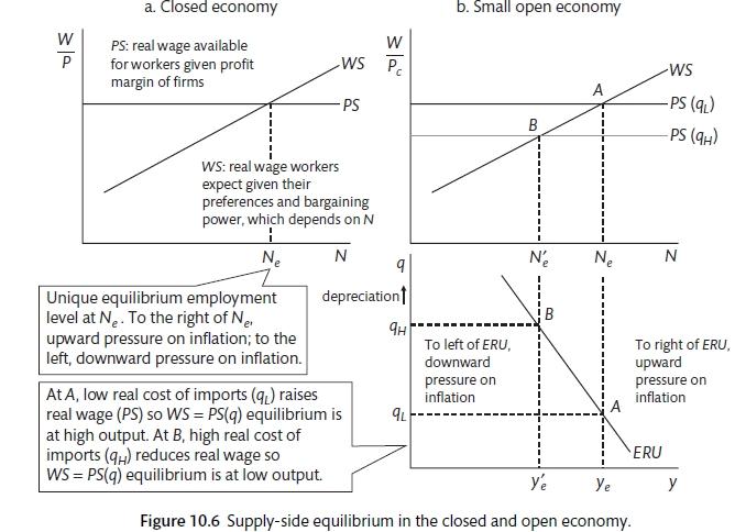
For a vertical ERU curve it is necessary to assume that workers are only interested in domestic prices. Now we look at the case where the WS curve is defined in terms of real consumer wages \((W/P_c).\) The y-axis on the WS curve will change as a result. The WS is still upward sloping as employment rises and the labour market tightens, the real consumption wage that workers can expect will increase. The WS curve is still affected by the labour market and things like the strength of trade unions and the availability of unemployment benefits. The PS curve is also defined in terms of real consumption wages \((P_c).\) Now PS is a function of the real cost of imports, it will shift upwards and downwards as the real exchange rate changes because depreciation reduces the real wage that workers get.
In this example there is a depreciation of the real exchange rate Q as a result of a depreciation of the nominal exchange rate e. The PS curve shows the real wages that workers get once they have set prices. With
\[P_c = (1 - \phi )P + \phi P^*e\]
there will be an increase because of the rise in e. In addition, as firms set their price as a mark-up on costs \((W/\lambda),\) the real exchange rate does not come into this calculation and therefore P does not change. P_c rises and the PS curve shifts downwards. The PS curve shows the real wages that are available to workers after firms have secured their profit-margin. It is also possible to think about the effect of import prices on firm costs. For now it is assumed that there are no intermediate goods. ASIDE: this is much less true than it was due to global supply-chains. As the PS curve shifts downwards, the equilibrium with the WS curve is at a lower level of employment. As a result, there is a negative relationship between the real exchange rate and employment and the ERU curve slopes downwards. It is possible in this model to have high employment and high output as long as the exchange rate is appreciating and raising real wages. However, a depreciating exchange rate will tend to work in the positive direction raisin inflation and the real wage rate will reducing employment.
Import prices and the labour market (Carlin and Soskice 2015)
Wage and price setting in the open economy.
\[P = P_x = (1 + \mu) \times \frac{W}{\lambda} \]
where \(\mu\) is the markup, the consumer price is defined as
\[P_c = (1 - \phi)P + \phi P^*e\]
as \[P_M = P^*e\]
The real consumption wage is
\[w = \frac{W}{P_c}\]
wage setting the same but the price level is defined.
\[W = P_c b(N)\]
So the wages setting real wage equation is
\[w_WS = \frac{W}{P_c} = b(N)\]
In the absence of intermediate goods, price setting in the open economy is the same as that in the closed.
\[P = P_X = (1 + \mu)\frac{W}{\lambda}\]
where \(\lambda\) is the leve of labour productivity.
The price setting curve must be expressed in terms of the consumer price index
\[P_c = (1 - \psi)P + \psi P^*e\]
so
\[P_c = (1 - \psi) \left [ (1-\mu)\frac{W}{\lambda} \right ] + \psi P^*e\]
\[W_PS = \frac{\lambda(1 - \mu)}{1 + \psi(Q - 1)}\]
or approximately
\[W_PS = \lambda(1 - \mu)(1 - \psi(Q - 1))\]
The wage-setting real wage in the open economy is equal to the closed economy price-setting wage \((\lambda(1 - \mu)\) modified by the real exchange rate and they are the same if the overseas part of the consumer price index is zero.
##The medium-run model Is created by the combination of the ERU, AD and BT curves in q-y space.
The open economy IS equation is
\[y_t = A_t - ar_{t-1} +bq_{t-1}\]
The AD curve is
\[y = A(\sigma, y^*) - ar^* + bq\]
where \(r^*\) is the real world interest rate and the constant A includes \(\sigma\) and \(y^*\) as shift variables.
For the economy to be on the AD curve, $r = r^* $as the real exchange rate must be equal to its expected value in equilibrium.
The medium term BT curve shows the combinations of the real exchange rate (q) and output (y) where trade is balanced.
\[BT = B(\sigma, y^*) + cq\]
B is a constant that includes the exogenous determinants of exports and imports.
BT is flatter than AD (c > b) as a rise in competitiveness improves the trade balance because of the Marshall=Learner condition and the fact that the multiplier is less than the inverse of the marginal propensity to import.
We will look at the way that the downward sloping ERU curve affects the medium-term effect of demand and supply shocks. A positive supply shock (such as a reduction in union bargaining power) shifts the WS curve downwards. This shifts the ERU curve to the right: the exchange rate depreciates and output rises. The improved competitiveness has moved the economy to a position of surplus. A positive demand shock (such as a fall in the savings rate) shits the AD curve to the right and leads to an appreciation of the real exchange rate. The economy has moved to a position of deficit. It is also possible to model the effect of shocks from outside the home economy. These could include changes in world demand or changes in the home country share of world exports. Either of these would shift the AD and BT curves to the right. These may come from a change in preference for wine over beer, increasing the share of French exports in the world economy, or an increase in the quality cars produced in India. The AD curve shifts to the right because \(A(\sigma, y^*)\) has increased and BT shifts to the right because \(B(\sigma, y^*)\) has increased. There is a real appreciation and, an increase in output and a move to a trade surplus. Table 10.1 assess the effect of a variety of exogenous shocks.
Inflation For medium term inflation stability the real exchange rate should be at equilibrium. Therefore we can say that \(\frac{\Delta Q}{Q} = 0\) and
\[\frac{\Delta Q}{Q} = \frac{\Delta P^*}{P^*} = \frac{\Delta e}{e} - \frac{\Delta P}{P} = 0\]
\[\frac{\delta P}{P} = \frac{P^*}{P^*} + \frac{\Delta e}{e}\]
This implies that the medium term inflation is determined by
\[\pi^{MRE} = \pi^* + \frac{\Delta e}{e}\]
Inflation is equal to world inflation plus the depreciation of the exchange rate.
If home inflation is \(5\%\) and world inflation is \(3\%,\) competitiveness will remain constant as long as the exchange rate depreciates at \(2\%\) per year. It is the monetary policy regime that determines the domestic inflation, so long as the policy is credible. This means that if the domestic and international inflation is determined exogenously, the nominal exchange rate will depends on the difference between the two. In a fixed exchange rate regime, the domestic inflation target must be the same as world inflation. The EMU is an example of a fixed exchange rate regime. The ideas was began in 1992 with the Maasstricht Treaty. This helped to anchor inflation expectations. This can be seen as a method of gaining credibility that is similarr to that of granting central bank independence.
[Medium Run Supply and Demand Shocks (Carlin and Soskice 2015)](./Figures/OpenSD/MedShocks.jpg]