Chapter 1 Demand
1.1 Learning outcomes
At the end of this chapter you should be able to
Identify the components of demand and the factors that affect their behaviour
Report key facts about the business cycle
Derive and use the IS curve
Explain the paradox of thrift
Understand the strengths, weaknesses and use of the Permanent Income Hypothesis (PIH)
Discuss the importance of credit rationing for the working of the PIH

Demand
1.2 Aggregate demand
This chapter builds the model of aggregate demand (AD). Aggregate demand is made up of household or consumer spending (C), business investment (I), government spending (G) and net exports (NX). It is about the spending decisions of households, firms and government. These decisions are complex but we will try to simplify by using a model. The model will attempt to capture the essence or most important features of the process. The economic decisions that we will consider will involve static and inter-temporal choice. That means making decisions about spending and saving now based on current conditions and based on expectations about the future. Therefore, we will eventually need a way of understanding how expectations are formed.
There is a role for the government. Government policy can influence aggregate demand: interest rates can affect spending decisions of households and investment decisions of firms as well as the exchange rate; taxation can change prices to be paid and income while government spending directly influences demand. People in other countries influence overall demand with purchase and production of goods and services. Figure 1.0 show the weights and the evolution of the components of UK demand over time. It is clear that consumer spending is the largest part of GDP but that business investment is more volatile.

GDP Components (Carlin and Soskice 2015)
The relative importance of these GDP components can change over time and can change between countries. Household spending or consumption is always the most important element of GDP. However, while consumption makes up 70% of GDP in the US, it is only 48% of the Chinese economy. An exceptionally high proportion of GDP in China comes from investment spending. This is a result of China’s drive to increase the amount and quality of capital in the economy.
| Country | Cons | Inv | Gov | Net Ex |
|---|---|---|---|---|
| China | 48.0 | 37.5 | 15.1 | 2.9 |
| Germany | 58.6 | 18.7 | 19.0 | 3.5 |
| Japan | 57.1 | 23.7 | 17.7 | 1.4 |
| United Kingdom | 65.3 | 16.7 | 20.0 | -2.5 |
| United States | 69.9 | 19.0 | 15.3 | -4.5 |
Figure 1.2: The share of expenditure components in GDP 2000-2005
The national accounts measure GDP and can be determined in three ways. This is an identity, meaning that it must be the same by definition. It is like cutting a cake in different ways, you still have the same cake no matter whether it is cut into three or four or five or whether you call it ‘cake’ or ‘tea’ or ‘desert’.
- Expenditure: this measures all the spending in the economy
\[y \equiv C + I + G + (X - M)\]
There are tricky decisions about which category some things should fall into. The purchase of a new house would fall into investment. Government transfers (benefits, pensions etc) are recorded as consumption when spent.
- Output: all the goods and services produced by the economy.
\[y \equiv \text{value of output sold - cost of raw materials and intermediate goods}\]
How do you measure the output of the health service?
- Income \[y \equiv \text{wages and capital}\]
The major part of this is wages. Capital is divided into interest, profits and dividends
As you can see from Figure 1.0, Investment is much more volatile than consumption or government spending. Investment is pro-cyclical. That means that it is strong when the economy is doing well and is weak when the economy is weak. Though usually having a relatively small share of GDP, business investment is therefore a key driver of the business cycle. Consumption is much larger but changes less as peoples’ spending habits are quite fixed. Nonetheless, these small changes in household spending can have a large effect on the overall economy. As the negative fluctuation becomes more extreme we get what is called a recession. In the US, the NBER makes the official definition of recessions. There is a popular notion that a recession is defined as two quarters of negative growth. However, not all recessions have negative growth so that is more of a rule of thumb than a strict rule.
The NBER reported on the 8 June 2020 that the US entered a recession in February 2020. This was the quickest announcement ever made.
On June 8, the NBER Business Cycle Dating Committee (BCDC) officially announced that the peak of the U.S. recession was reached in February 2020. Some previous Econbrowser posts already suggested that February was indeed the end of the longest economic expansion in history (128 months),
You can read more about this on the [Econbrowser blog](http://econbrowser.com/archives/2020/06/guest-contribution-a-severe-us-recession with a fuller discussion of identifying recessions.
It you read that article, you will see that the current recession and what is called The Global Financial Crisis (GFC) of 2007-08, are the two largest recessions on record. These two major econonic shocks come after a period that was called The Great Moderation due to the relative stability of the economies of developed nations. You can see this from Figure 1.2 where the rolling standard deviation of GDP is recorded.
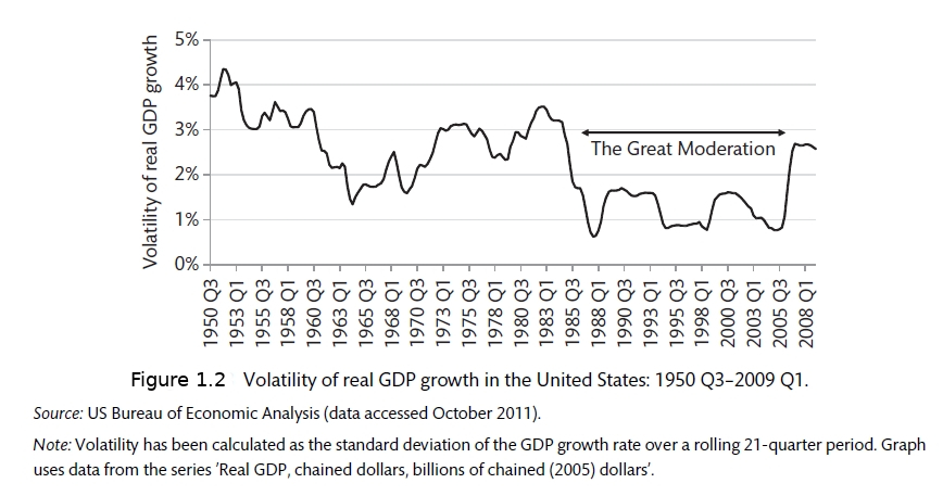
The Great Moderation (Carlin and Soskice 2015)
Some people believe that there is a realtionship between periods of economic calm and major shocks. The Great Moderation proceeded the Global Financial Crisis (GFC). We will discuss in detail in chapters 4 and 5 how these two events may have been related. The calm conditions made people complacent.
There are of course many questions raised about the use of GDP as a measure of welfare. You can read about some of these limitations here
1.3 The New Keynesian model
Aggregate demand is the first part of the New Keynesian model that we will consider. Models are important in providing a framework for thinking about complex problems. This model represents the three key elements of the complex macro world. The first tries to capture demand, the second assesses supply and the third brings together policy and the Phillips Curve. Aggregate demand is represented by the IS curve and refers to the combination of planned investment and savings decisions that are consistent with equilibrium in the market for goods and services. The IS framework summarises the way that changes in spending decisions of households, firms and government are affected by the level of real interest rates and the way that they multiply through the economy.
We begin with the Keynesian Cross. You can refresh your knowledge of this model by going back to the Section on Fiscal Policy in the CORE Textbook. The economy operates are equilibrium where spending is equal to output (the 45 degree line). If this is not the case, the economy is not in equilibrium and there will be an incentive for firms to change their behaviour.
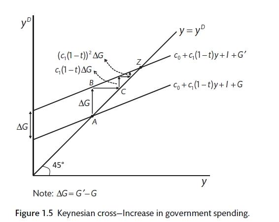
The Keynesian Cross (Carlin and Soskice 2015)
Figure 1.3 shows the Keynesian Cross. This is the source of the IS curve. If spending and output are not equal, there is either excess demand or demand is too low. In either of these cases firms will take action to return output to the level of planned spending by increasing or decreasing the amount that they produce. If demand is too low, as it has been during the outbreak of Corvid-19, firms will cut output by curtailing overtime and hours worked or even making people redundant. This has secondary effects as people with lower income now spend less. In this case, the economy circulates downwards until output and demand are equal again. The feedback of lower income onto lower spending and the interaction between the two is called the multiplier.
Please follow this link to the Keynesian Cross. The economy will begin at equilibrium where GDP is equal to £30.0 million. Autonomous household spending, business investment and government spending are all equal to £2.0 million. If we envisage an increase in government spending to £4 million, you can see the effect on the economy. A £2.0 million increase in government spending can increase the size of the economy by £10.0 million. This is the multiplier.
1.3.1 Exercise 1.0
- Assume that a cut in interest rates increases business investment to £4 million from its current £2.0 million. What is the effect?
- If households are worried about the future and cut back autonomous spending to £1.0 million, what is the effect on the economy?
1.4 The IS curve
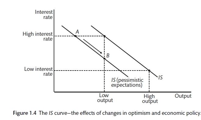
From the answer to question 1 above, we can draw the IS curve and the relationship between interest rates and aggregate demand. It is downward sloping, suggesting that lower interest rates lead to higher aggregate demand. This is controversial. Interest rates are believed to affect household spending (through mortgage, house purchase and the purchase of furnishings as well as making savings more attractive. Interest rates also affect the feasibility of investment project for firms. Lower interest rates make it cheaper to borrow. However, firms may also be affected by their expectations for the future. As we will see in Chapter 10, interest rates can also affect the exchange rate and therefore imports and exports.
The IS curve shows the combination of interest rates and output for which aggregate spending is equal to output. The market for goods and services is in equilibrium. The IS curve is downward sloping as high interest rates constrain spending by households and firms. When interest rates are low investment and household spending are high and GDP should also be higher. To show how changes in profit or income expectations can affect the economy, we need to shift the IS curve: more pessimism will shift the IS curve inwards meaning lower business investment at each level of interest rates. Government spending will also shift the IS curve. This could be used to counteract the increased pessimism. There is much debate over the effect of government spending on overall output. A key question in macroeconomics is, What is the size of the ‘multiplier’?
The IS curve
The IS curve will be built on the basis of consumption demand, investment demand and demand from government purchase. For now we have a closed economy with no trade with the rest of the world.
Aggregate demand is given by
\[y^D = C + I + G\]
All variables are in real terms or constant price. Equilibrium requires that planned spending (aggregate demand) is equal to output.
\[y^D = y\]
Consumption is a linear function of disposable (after-tax) income. Here \(c_1\) is called autonomous spending. This is spending that does not depend on income. \(T\) is the amount of tax and \(c_1\) is called the marginal propensity to consume (MPC). The MPC shows how much of an increase in income is spent.
\[C = c_0 + c_1(y - T)\]
Where T is tax net of transfers.
To get the consumption function, we assume that taxes are a fixed proportion of income so that \(T = ty\) and \(0 < t < 1\). Therefore t is the tax rate. Now,
\[C = c_0 + c_1(1 - t)y\]
This is the Keynesian consumption function. \(c_0\) is autonomous consumption and the rest shows that household spending is a fixed proportion of disposable income and \(c_1\) is the marginal propensity to consume.
\[MPC = \frac{\Delta C}{\Delta y^{dis}} = c_1\]
Where \(y^dis = (1 - t)y\)
In this model of consumption (or consumption function), saving is \(S = y - C\) and adds to household assets. Income is the amount that can be consumed without depleting assets. The marginal propensity to save is \(s_1\). Therefore, \(s_1 + c_1 = 1\).
Savings are determined by desire to smooth consumption over time (see below) and for precautionary reasons. The second of these is likely to change when people become worried about the future. (Moody, Ohnsorge, and Sandri 2012) uses a panel of 27 countries to show that a 1 percentage point increase in the unemployment rate increases the savings rate by an average 0.3 percentage points. You can read more about the way that the recovery from the Covid-19 shutdown may be affected by precautionary savings on the Econbrowser blog post by Bank of Italy Directory General for Economics, Statistics and Research Valerio Ercolani.
1.4.1 The multiplier
If the consumption function is substituted into the equation for aggregate demand, it is possible to get the relationship between aggregate demand and output.
\[y^D = c_0 + c_1(1-t)y + I + G\]
In aggregate demand, output space, this line and the 45 degree line for equilibrium can be drawn. The working of the model can be demonstrated by disturbing the equilibrium by (say) an increase in government spending. This will shift the AD line parallel to the original. Output will increase to meet demand (as inventory systems indicate that there is a shortfall), raising income and demand with second round effects. It is possible to find the find equilibrium in terms of exogenous variables by substituting output \((y)\) into aggregate demand \((y^D)\).
\[y - c_0 + c_1(1 - t)y + I + G\]
\[y - c_1(1 - t)y = c_0 + I + G\]
\[y = \underbrace{\frac{1}{1 - c_1(1-t)}}_{\text{Multiplier}}\underbrace{[c_0 + I + G]}_{\text{Autonomous}}\]
This the multiplier and autonomous demand. As \(c_1\) and t are between 0 and 1, this means that the multiplier must be greater than one. This is the short-run multiplier where interest rates and all other policy responses do not change. If the mpc is zero, there is no multiplier.
It can be shown that the sum of a geometric progression is given by
\[\Delta y = \frac{1}{1 - c_1(1 - t)} \Delta G = kG \]
With k as the multiplier.
The paradox of thrift says that saving in a recession will not be beneficial overall. It is possible to model the effect of a proposal to encourage savings during a recession by reducing \(c_0\) to \(c_0^1\). Aggregate demand will fall by the difference between the two and the multiplier process will work in a downward direction. Indeed, the attempt to increase savings will not be successful.
\[\Delta S = \left [ (1 - c_1(1 - t)) \frac{1}{1 - c_1(1 - t)} \Delta c_1 \right ] - \Delta c_1 = 0\]
The paradox of thrift is that if the increase in savings is not met by an increase in investment, there will be no overall increase in savings in the economy. Using this model, it is clear that encouraging savings is not a good idea if the economy is in a recession. There is no mechanism in this model whereby higher savings are translated into higher investment.
1.5 The real interest rate
t is assumed that aggregate demand is influenced by the real interest rate.
\[r = i - \pi^E\]
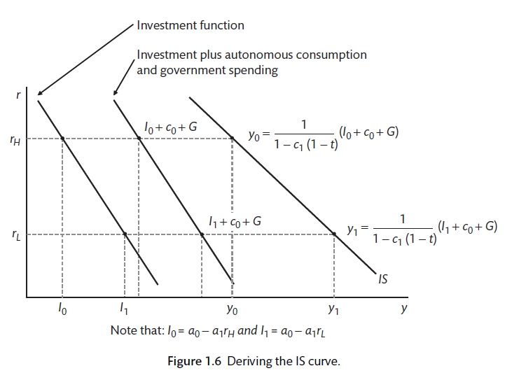
The real rate is the nominal rate adjusted for inflation expectations. The real rate is the one that is used in the IS curve. When the central bank sets its interest rate it changes the nominal rate to obtain a particular real rate that it believes will affect the economy. For now we assume that there is just one interest rate in the economy. For now consumption is independent of interest rates. Therefore, interest rates work through the effect on investment spending, including the purchase of new houses. Up to now we assume that investment is set by expected future profits, which are exogenous. Now the investment function is
\[i = a_0 - a_1r\]
\(a_0\) is autonomous investment. It is investment that does not depend on real interest rates. Expected future profits are captured by \(a_0\). The relationship between investment and the real interest rate is denoted by \(a_1\). It is less than 1. Now substitute this investment function into the IS curve
\[y = \frac{1}{1 - c_1(1 - t)}[c_0 + a_0 - a_1r + G]\]
\[y= k[c_0 + (a_0 - a_1r) - ka_1r\]
To simplify,
\[y = A - ar\]
Where \(A = k(c_0 + a_0 + G)\). These are all the autonomous elements of spending that are exogenous or determined outside the system. Now, \(a \equiv ka_1\). This highlight the fact that for a given interest rate, equilibrium is determined by the multiplier of autonomous spending elements. A higher multiplier or a more sensitive response from investment interest rate changes, the more effect interest rates will have on output.
IS curve
1.6 Permanent Income Hypothesis
Expectations are important for firms and households. There is an intertemporal element to household spending and business investment. Decisions that are taken across time. Households will adjust their spending to expected future income. Business make investment decisions based on expectations about future demand for products and input costs. Borrowing against future income is called consumption smoothing. People would like to smooth their consumption over time so that they do not have times when the consume excessively and other times when the consume little. You can return to the CORE Textbook to revise the information about the borrowing, lending and consumption smoothing.
I is possible to model the expected present value of future household income. If we assume that people do not die, this would be the present value of wealth based on current wealth and expected future income. The imortality assumption makes the math easier and can be justified by talking about households where people die and pass any wealth on to their children.
\[\Psi_t^E = (1 + r)A_{t - 1} + \sum_{i = 0}^\infty \frac{l}{(1 + r)^i} y_{t - i}^E\]
Where y is the post-tax income, discounted back to today for each year until infinity and A are the assets or wealth at the beginning of the process.
Household consumption has to take account of the smoothing of consumption over periods when income may rise and fall due to expected and unexpected outcomes. The smoothing of consumption is based on the diminishing marginal utility of consumption. The Permanent Income Hypothesis (PIH) suggests that individuals optimally allocate their consumption over their lifetime. The resources used for this include assets and future income. This comes originally from (Modigliani and Brumberg 1954) and (Friedman 1957). Figure 1.7 shows how income and consumption change over the time in a simplified model. In general, there is savings when people are young, savings at the prime earnings time of life and then savings are run down during retirement. The government can also play a part in this process by providing benefits and social insurance. The greater the government involvement, the less there is for the private sector to do.
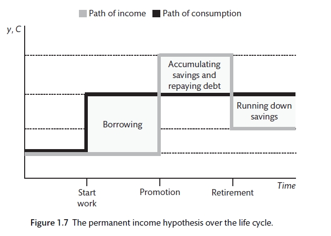
Permanent Income Hypothesis (Carlin and Soskice 2015)
This model of consumption is different from the Keynesian version where the future is not explicitly considered. The question of whether individuals would like constant consumption or gradually rising or falling consumption will depend on the rate of interest \((r)\) and the rate at which individual trade assess the benefit of consumption now relative to consumption in the future. The second of these is represented by \(/rho\) which is a measure of impatience. The household chooses a part of consumption to maximise lifetime utility subject to the budget constraint.
\[\Psi_t^E = (1 + r)A_{t-1} + \sum_{i - 0}^\infty \frac{l}{(1 + r)^i} y_{t-1}^E\]
This can be simplified to a choice about consumption in the current period and consumption in the future. This can be represented by the Euler equation.
\[C_t = \frac{1 + \rho}{1 + r}C_{t + 1}^E\]
If the interest rate \((r)\) and the subjective discount rate \((\rho)\) are the same, the benefit from savings will be equal to the gains from saving and consumption will be constant so that \(C_1 = c_{t + 1}^E\). If the discount rate is above the interest rate \(C_t > C_{t +1}^E\) so that consumption is falling overtime and if the discount rate is lower \(C_t < C_{t + 1}^E\) so that consumption is declining over time. It is easiest to focus on cases where the subjective discount rate is equal to the interest rate. The PIH consumption function is
\[C_t = \frac{r}{1 + r} \Psi_i^T\]
Where \(\Psi_i^T\) is the present value of the discounted value of expected future income (as derived above). This remains constant unless expected wealth changes. In contrast to the standard Keynesian consumption function outlined above, you can see that a change in expected income should have no effect on spending. An unexpected change in income will have only a small affect on spending. For example, if the interest rate \((r)\) is \(4\%\) the effect will be i
\[\frac{r}{1 + r} = \frac{0.04}{1.04} = 3.8\%\]
In that case a £100 million increase in government spending will increase output by just £104.0 million.
Going back to the multiplier, the MPC is just 3.8% (as above).
\[\Delta y = \frac{1}{1 - c_1(1 - t)} \Delta G = kG \]
\[k = \frac{1}{1 - 0.038} = 1.04\]
A temporary increase in income will have a much more modest effect because it will be spread over the entire future in the attempt to smooth consumption.
There are two prediction of PIH that do not seem to found fully in practice:
- That people will borrow to smooth consumption if they are expecting earnings to increase in the future. In reality, earnings seem to be excessively sensitive to income. Spending does not seem to increase until income actually increases, even in cases when an increase in income can be strongly expected.
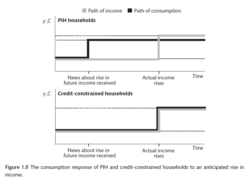
Excess sensitivity
- That people will anticipate retirement and will reduce their spending before they get to that date. However, spending seems to more sensitive to actual retirement that would be forecast from this model. This is quite surprising as it relies on saving rather than borrowing and therefore is not affected by credit constraints.
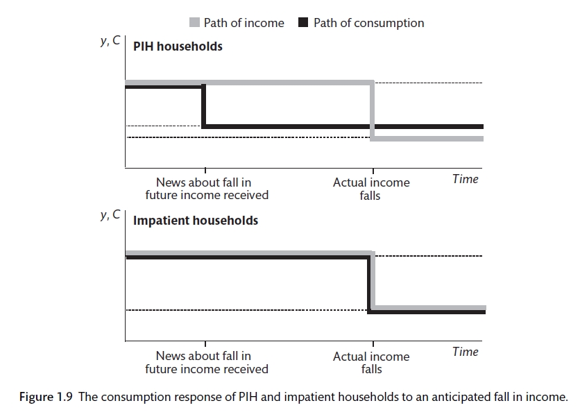
Excess response
There are three major reasons why PIH does not hold: credit constraints; impatience; uncertainty about future income. There are a number of empirical studies that have been carried out. (J. Y. Campbell and Mankiw 1989) tested the sensitivity of consumption and income from G7 countries. They found that consumption is sensitive to income,. It rejected PIH. (Johnson, Parker, and Souleles 2006) found that the average US household spent 20% to 40% of the temporary (one-off) tax cut within three months of it being received, rather than when the programme was announced. Random social security numbers were used to distribute gains. Households with low income responded most suggesting that credit constraints are important. Spending falls with retirement but this could be because there is a cut back in job-related spending (Jappelli and Pisaferri 2010). There is ample evidence that people are more impatient (higher discount rates) that the PIH would suggest. It is likely that households find it hard to determine whether a change in income is permanent or temporary.
#Supply ## Learning outcomes At the end of this chapter you should be able to
- Understand and use the WS-PS model
- Explain the properties of the Phillips curve and discuss why this relationship has become weaker in recent years
- Analyse the determinants of medium term unemployment
- Outline the economic consequence of divergence from medium-term equilibrium

Work
Supply is about firm decisions concerning the level of output, employment as well as wages and prices. The labour market does not appear to work like a traditional market that are determined by supply and demand. Unemployment is characteristic of a capitalist economy. Workers are willing to work at the prevailing wage rate but cannot find a job. Across the world this is happening but the supply-demand model suggests that the wage will fall to clear the market. Unemployment varies from country to country and across time, so it is clear that the business cycle and institutions can affect the number of people without a job. The unemployed are not happy to be without a job. (Clark and Oswald 1994) found that unemployed workers have twice the amount of mental distress as the employed. This is not volentary unemployment.
1.7 Why do labour markets not clear?
The New Keynesian model uses an efficiency wage model for the labour market (Carlin and Soskice 2015). This allows us to explain unemployment and the failure of wages to clear the labour market. The supply of labour is determined by the wage setting (WS) curve. The higher the wage, the more willing people are to work. The demand for labour is shown by the price setting (PS) curve. Firms offer wages based on the level of productivity, the level of competition, taxes and other factors. You can revisit the CORE textbook for more details on the labour market supply model.
Efficiency Wage model (Carlin and Soskice 2015)
The efficiency wage idea was first proposed by (Shapiro and Stiglitz 1984) in a paper called Equilbrium Unemployment as a Worker Discipline Device.
The model for the supply side of the economy is also based on monopolistic-competition where firms have market power to set prices. There can be changes in the level of competition based on the number of firms in an industry. The greater the market power, the more firms are able to increase their mark-up or profit margins. At the extremes, there are perfectly competitive and monopolistic markets.
It is assumed that wages and prices are not adjusting continuously but are changed infrequently. (Barattieri, Basu, and Gottschalk 2010) analysed wage setting in the US and found that wages were sticky. A simple model would suggest that wages are set once a year. This does not appear to vary much across different industries. (C. M. Campbell and Kamlani 1997) surveyed 184 firms and found that most firms were reluctant to cut wages in a recession. Firms felt that they would lose their best workers. Firms also thought that it would damage moral and reduce effort. (Bewley 2007) review literature on wage rigidity and fairness and found that wage cuts were only perceived as being fair if they saved a large number of jobs. This may explain why wages do not tend to fall to clear the market during a recession. However, rigidities in price setting varies by industry.
Nominal wages do not adjust immediately to fluctuations in aggregate demand. Economic agents set wages and prices with a target real value that requires some assumption about future inflation. The real wage (w) is the nominal wage (W) deflated by the price level (P).
\[w = \frac{W}{P}\]
For this New Keynesian model, wages are set once a year during the wage round and prices are adjusted after that. Therefore, wages and prices adjust to aggregate demand with a lag. In this case a positive demand shock will lead to higher employment, lower unemployment and an increase in wages (as a move up the WS curve). Firms respond with an increase in prices. We assume that the mark-up or profit-margin is unchanged. All firms in the industry increase wages.
1.8 Changes in equilibrium unemployment.
Equilibrium unemployment will rise if the WS curve shifts upwards or the PS curve moves downwards.
An increase in unemployment benefits would shift the WS curve upwards. There is a trade off between the effect that an increase in benefits has on reducing the cost of job losses and the need to shift to a lower point on that wage setting curve to ensure productive output. This is achieved with a higher level of unemployment.
Higher mark-ups as a result of lower competition. The PS curve is reduced and a higher share goes to profits. There is less employment and lower real wages. This may be something to consider with recent examples. With the higher cost of job loss the real wage is lower.
Policies that shift the WS or PS curves will affect the level of equilibrium unemployment and the growth rate of the economy. These are supply side policies that we will focus on in Chapter .
1.8.1 Labour-supply
Analysis of the supply-side of the economy is broken down into two parts: supply-side effects on unemployment; nominal rigidities.
\[w = Pe B(N, z)\]
Where the wage \((W)\) is determined by the expected price level, the level of employment \((N)\) and a set of wage-push variables \((Z).\) This will include changes in benefits and the presence of unions.
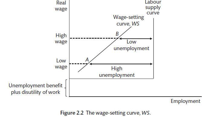
Though nominal wages are set or negotiated, works are interested in the real wage. The wage-setting (WS) real-wage equation is
\[w(WS) = W/Pe = B(N, Z)\]
The opportunity cost of taking a job is dependent on two factors: benefits and the disutility of working. The wage is above the opportunity cost of working and increases as the unemployment rate falls. As unemployment falls firms have to pay more to get people to work hard as there are lots of job opportunities. There are a number of enhancements that can be applied, including adding monopoly unions. As such, changes in institutions can affect the WS curve and the equilibrium level of unemployment.
1.8.2 Labour-demand
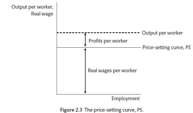
In a competitive market the firm sets prices and the quantity of labour required with reference to the marginal product of labour. In this case \(P = MC and W/P = MPL\). However, once there is market power, as is the case with our assumption of monopolistic competition, firms facing a downward-sloping demand curve will produce to maximise profits. The mark-up on marginal cost will be depend on the elasticity of demand, which will be influenced in a positive direction by the level of competition. As elasticity rises the mark-up will fall. A horizontal PS curve is usually employed, if firms set prices according to a mark-up over costs. Now the fixed output per worker is split between profit per worker and the real wage per worker. The real wage is the marking-up of unit labour costs by a fixed percentage \((\mu)\).
Therefore,
\[P = (1 + \mu)(W/\lambda)\]
Where \(\lambda\) is output per worker \((y/N)\).
Output per worker is divided into real wages per worker and real profits per worker.
Productivity, prices and wages
There is a divergence between the real consumption wage (based on post-tax income and excise duties prices) and the real product wage that is paid by the employers - including income tax and other taxes relative to the price that is received for product after indirect taxes are paid. The difference is the tax wedge. The tax wedge is one of the price-push factors that may affect the PS wage.
\[W^PS = \lambda F (mu, z)\]
Changes in productivity, competitive conditions and taxation can change the price-setting wage. Other price-push factors are business regulations and employment relations, Some health and safety regulations may impose costs but provide an offsetting increase in productivity.
Labour market equilibrium is at the intersection of the upward sloping WS curve and a flat or downward sloping PS curve.
\[W^ws = W^ps\]
\[B(N, z_w) = \lambda F (\mu, z_p)\]
1.9 Exercise
Please go to the labour market app and make the following adjustments:
An increase in productivity
A reduction in benefits
An increase in competition
Make sure that you are happy with the model and the adjustments to real wages, employment and unemployment that each of these changes would suggest. In what ways is the model unrealistic? How can we account for that? How would those changes affect the model?
1.10 The labour market and the business cycle
Nominal rigidities describes the way that wages and prices fail to constantly change and clear the market. A model where workers demand wage changes based upon the level of unemployment and firms accept these wage changes and then adjust prices so that the mark-up over costs is maintained is supported by empirical evidence (Alvarez et al. 2006). As a result, employment will change with the business cycle - rising when the economy is strong and falling when it is weak. Firms often set prices strategically in relation to the behaviour of other firms in the industry.
Okun’s Law studies the empirical relationship between unemployment and output. The relationship may be affected by labour hoarding and by movement into and out of the labour force. A 1% change in output above or below its long run trend has an effect of 0.5 percentage points on the unemployment rate. This is different for different countries. A formalisation of the link between unemployment and inflation is the behavioural model called the Phillips curve. This can be written as
\[W^ws(y) = (W/P)^ws = B + \alpha (y_t - y_e) + z_W\]
Where B is a constant that reflects unemployment and the disutility of work while Z_W is a set of cost-push factors, \(y_t\) is the level of output or GDP and \(y_e\) is the equilibrium output associated with the natural or long-run level of unemployment.
1.11 The Phillips curve
You can revisit the CORE discussion of the Phillips curve. In the New Keynesian model, the Phillips curve is pinned down by lagged inflation because lagged inflation is a key component of the wage inflation mechanism. This is because we assume that inflation expectations are based primarily on the past performance of inflation. We will use adaptive wage expectations. When determining the wage that they will accept, workers look at past inflation as their guide to the future. We can adjust this assumption if necessary.
This is the adaptive expectations Phillips curve.
\[\pi_t = \pi_t^E + \alpha (y_t - y_e)\]
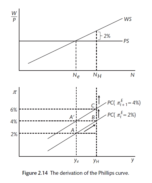
The Phillips curve (Carlin and Soskice 2015)
1.12 Demand and supply shocks
We can use the components that we have of the New Keynesian model to discuss the effect of demand and supply shocks. The demand shock could be the fall in spending that has been caused by the Covid-19 lockdown or by an increase in household spending due to increased confidence about the future. The IS curve shifts, the increased demand and output causes a disequilibrium in the labour market and inflationary or deflationary pressure. There is nothing to stop inflation rising or falling in without intervention from the central bank.
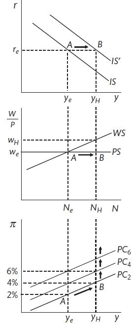
A demand shock (Carlin and Soskice 2015)
There are a number of factors that could produce a supply shock: technology or productivity shock \((\lambda)\), a shift in worker bargaining power (WS) or a change in level of competition amongst firms(PS). UK labour market reforms of the 1980s included reducing trade union power, making it more difficult to apply for unemployment benefit and reducing the level of benefit. These have the effect of shifting the WS curve to the right and reducing the equilibrium level of unemployment.
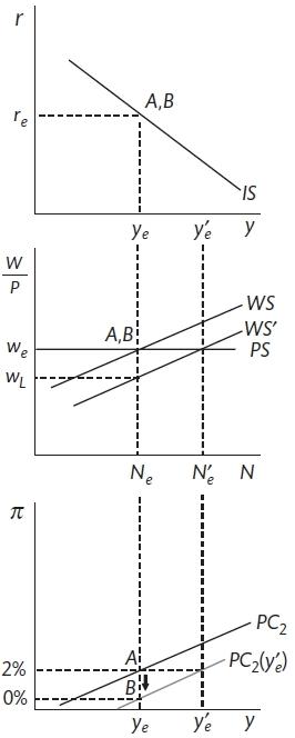
A supply shock (Carlin and Soskice 2015)
A shift in the WS curve means that employment at \(N_e\) is below the new equilibrium of \(N_e^1\). This will cause workers to accept lower wage increases and for inflation to fall as these cost changes feed through into prices. The process will unless demand and output can increase employment to the new equilibrium.
1.13 The post-Covid world
The post-Covid world appears to be suffering from the combination of a simultaneous demand and supply shock. Demand has increased as people have been able to purchase goods and services such as holidays, clubs, evenings with friends that were previously banned. This is likely to dissipate somewhat. However, there may also have been a shift to the left in the Wage Setting (WS) curve as people reassess their life-leisure balance, find it hard to get childcare and find that new ways of working. The Price-setting curve may also have been affected by the change in working practice that the lockdown encouraged. How long these supply-side changes persist is much less clear as are the longer term consequences of the more flexible on-site to remote working practices. The immediate picture seems to be a leftward shift in equilibrium unemployment and a rightward shift in demand that has left a shortage of workers and upward pressure on wages.