Chapter 5 The Global Financial Crisis
By the end of this chapter students should understand
The pre-crisis conditions that caused the Global Ginancial Crisis
The events and mechanisms that contributed to the elevated financial cycle
The effects of the crisis
The link between the GFC and the New Keynesian model
The policy interventions
In the 1990s and into the new century, there was a sense of complacency as the new macroeconomic regime seemed to have removed the threat of inflationary and unemployment shocks. Household debt rose by 8 percentage points between 1988 and 1998, and 29 percentage points between 1998 and 2008; financial debt rose by 29 percentage points 1988 and 1998 and 48 between 1998 and 2008. Central banks did little to prevent the build up in debt. US Fed Chairman Greenspan promoted a view that the central bank should concentrate on moping up the aftermath with low interest rates to maintain a dynamic economy. The focus was on inflation. However, the BIS pointed out the there are period when inflation can be low but rising debt can cause risk of disruption (Borio and White 2004).
5.1 Pre-crisis system: incentives, instruments and actors
By neglecting the social cost of its own bankruptcy, a financial firm will tend to take on more risk than is optimal. The brief that strategically important institutions will be bailed out reduces their cost of capital and encourages them to lend more and to take on more risk than they would otherwise. Banking sector gains are privatised while the losses are at least partly socialised. Lower regulation, lack of concern at the increase in risk and idea that new institutions had reduced the risk of macroeconomic shocks also increased the risk that was built up in the economy. There are a number of factors that contributed to the increase in financial frailty in the period after 2000. These included new financial instruments, expansion of the rating agencies and complacency. There are three instruments at the heart of the crisis: mortgage bonds, Collateralised Debt Obligations (CDO) and Credit Default Swaps (CDS). Rating agencies provide ratings for bonds issued by firms. They expanded their operations so that they rated other securities, including mortgage bonds and CDOs. The ratings run from triple A (AAA) down through Bs and Cs. The last of these are called non-investment grade, high yield or junk. High quality triple A assets do not require equity or capital to be held against potential losses. Therefore, the higher the credit rating of securities held by banks, the higher the return on equity (a key metric for investors). There was also an increased interconnection and concentration in banking. This made the whole system more vulnerable.
The upswing: US government encouraged home ownership amongst the lower paid as a way to tackle poverty. There is an argument that says that support for sub-prime lending was a counter action to the fall in business investment after 2000 and the weakness of consumer spending as a result of stagnant real wages. This prevented the IS curve shifting to the left. Sub-prime mortgages extended credit to those previously constrained. Consistent with the financial accelerator more loans led to higher house prices and more lending and leverage. The higher the leverage the higher the returns and losses. Consumption functions have a strong wealth element in the US and UK. The transmission of risk across the globe was facilitated by light European regulation of housing assets, European government implicit guarantee for European banks. European banks could hold US mortgage assets with minimal capital backing. European banks were significant buyers of Mortage bonds and CDOs.
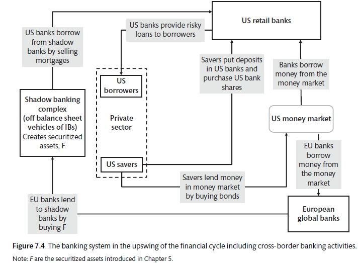
The Network of US and European banks (Carlin and Soskice 2015)
##The Credit Crunch (2007-08) The US central bank, the Fed, was raising US interest rates from late 2004 onwards due to the inflation risk caused by rising oil and other commodity prices. Higher interest rates eventually led to higher mortgage rates and started to dampen house prices rises. When house prices started to fall, negative equity (where the value of the loan is worth more than the value of the house) as the value of collateral started to fall. There was a rise in the default rate on home loans in February 2007. In August 2007 BNP Paribas stopped redemptions at some investments because it could not value its structured products. Short-term funding using housing securities as collateral became difficult. As financial tension increased other forms of collateral started to become less welcome and attracted larger haircuts. This is where more collateral is required for borrowing (in other words, you need $1.5m in mortage bonds to borrow $1.0 in cash, the gap between the two is the haircut). There was an increase in the spread between central bank money and the interbank rate. When CDO could not be valued and liquidity dried up parents had to fund the SIV that had been created. Northern Rock had only 23% of its funding from depositors in the summer of 2007. Bear Stearns was rescued in March 2008. On 15-September 2008 Lehman Brother collapsed.
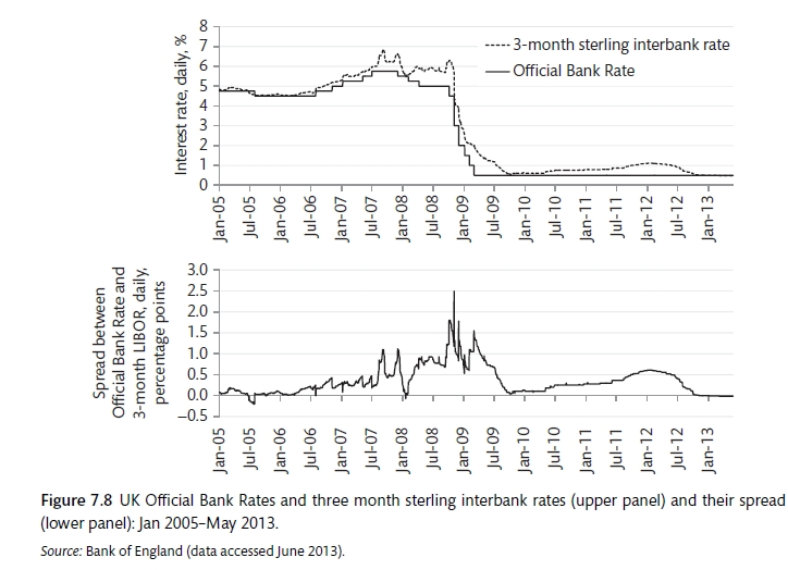
The spread between official rate and the policy rate (Carlin and Soskice 2015)
In these circumstances the policy rate loses effect because the spread between lending rates and policy rate increases; zero-bond also provides a constraint on the policy rate. Figure 7.10 shows the collapse using the three-equation model. The fall in the housing market causes a fall in consumption and housebuilding, shifting the IS curve inwards; central bank wants to cut rates but is constrained by the zero bound; even when the nominal rate is cut to zero, it is impossible to get the economy on the MR line at point C; the increase in the spread between policy rate and lending rate meant that economy was at point X rather than D with a lower level of output and falling inflation expectations; the fall in asset prices will increase the real debt burden for debtors and make de-leveraging more difficult and painful.
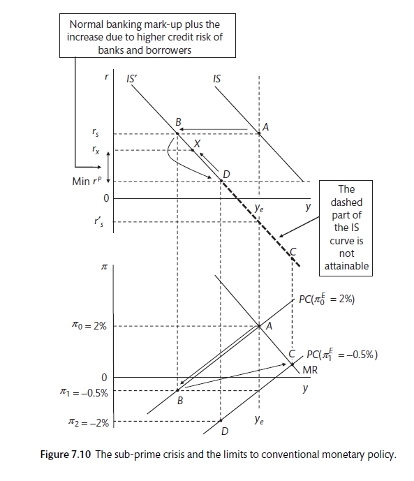
The collapse and the zero bound (Carlin and Soskice 2015)
5.2 The GFC compared to the Great Depression
The policy response to the GFC was build on some lessons from the Great Depression: maintain liquidity and avoid protectionism. There are a number of comparisons of the Great Depression and the GFC. World trade was more robust, production fell by a smaller amount, money supply was stable and budget deficit increased by more in the GFC. The Chair of the US central bank, Ben Bernanke address the issues of liquidity and bank solvency. Governments took ownership stakes and supported banks and tried to encourage restructuring of debt.
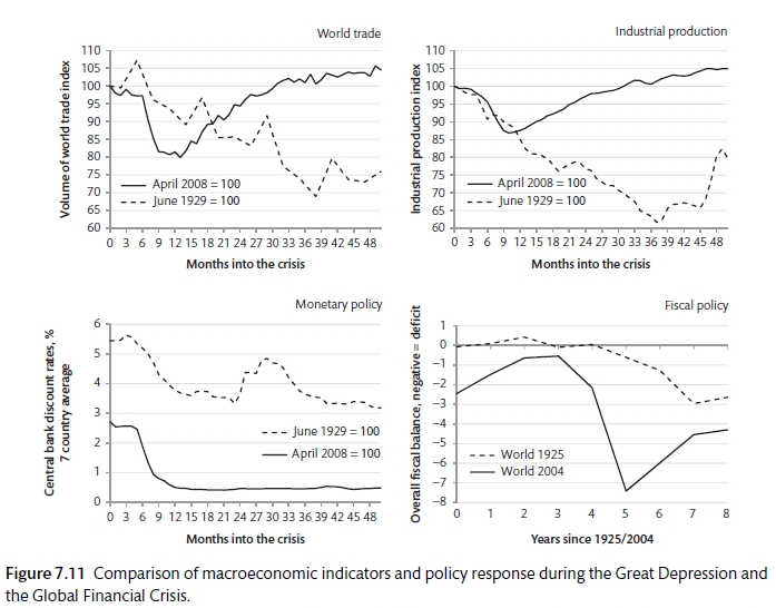
Comparison of GFC and the Great Depression (Carlin and Soskice 2015)
However, the GFC showed the limits of monetary policy. The zero-bound suggests that it is difficult to reduce interest rates below zero and that reducing real interest rates is difficult in times of deflation. As a result, central banks tried new monetary methods such as:
Quantitative easing (focusing on the quantity rather than the price of money)
Forward guidance (trying to manage expectations)
The way to deal with this is to use fiscal policy rather than monetary policy.