Chapter 2 Policy
At the end of the session you should be able to
- Understand the role of the central bank in inflation targeting
- Identify and use the Monetary Policy Rule (MR)
- Use the New Keynesian model to assess the effect of economic shocks
- Demonstrate how inflation is stabilised in the New Keynesian model

Balance
2.1 Modelling
The model is the simplification that allows us to say something about the working of a more complex system. This is a new-Keynesian model. There are also old-Keynesian, Real Business Cycle models. Different models will give different predictions. Therefore much of the macroeconomic and policy debate is about which is the most appropriate model. Real Business Cycle models do not have the sort of financial frictions or imperfections that were a large part of the Global Financial Crisis (GFC). You can read more about this in Chapter 16 of the (Carlin and Soskice 2015) text.
To complete the New Keynesian model we will look at policy or the monetary rule. Central bank policy is designed to stabilise the economy, preventing and an inflationary or deflationary spiral. There are a number of assumptions:
- The central bank wants to minimise the pain of allowing inflation to deviate from the 2.0% target while ensuring that unemployment does not move to far above the natural or NAIRU rate.
- The central bank is modelled as having rational expectations. This means that it uses our model to understand the economy. Compare this to the wage setters using adaptive expectations by looking backwards to determine what will happen to inflation in the future.
- The government will use monetary policy to stabilise the economy rather than fiscal policy
Figure 3.3 shows the Bank of England view of the way that monetary policy affects the economy. This is termed the monetary transmission mechanism.
The Monetary Transmission Mechanism
Monetary policy is preferred over fiscal policy because it is more immediate and it is less inherently political (though each of these can be questioned). There are many empirical exercises that can be carried out to show that inflation has become much more stable and less volatility since the implementation of the inflation-targeting regime. However, the post GFC world showed the limit to this policy: the zero bound and the risk of a deflation trap became evident. Some policy choices (such as a fixed exchange rate) can also limit the scope of the central bank to take these decisions.
The costs of inflation are mainly distributional. Inflation is generally good for those with debts and bad for those with credit. Inflation erodes the real value of a debt as income and revenue tend to rise with the nominal value of the debt is unchanged. Inflation may also distort incentives and cause inappropriate actions. Economists are concerned about inflation undermining the ability of prices to convey information. For example, if you get a large pay rise is it due to increased demand for your work or just the consequence of overall inflation. Important signals may be missed in a high inflation world. Central bank targets are around 2% to avoid deflation risks. Deflation at low levels is more damaging than low levels of inflation: debts become more of a burden and households delay consumption in anticipation of lower prices.
2.2 The model
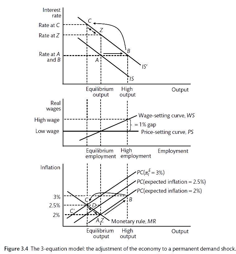
In a consumer boom, the following adjustments are found.
- There is a shift in the I-S curve as a result of an exogenous demand shock. This might be a rise in consumer spending due to increased confidence.
- Increased demand translates into higher output and employment.
- Wages increase by 3.0%, with a 2.0% compensation for inflation and a 1.0% increase due to increased employment. Workers see that there are plenty of jobs and demand higher wages. Firms see that they need to play more to attract workers.
- Firm immediately increase prices by 3.0% to protect their profit margins.
- There will be a shift in the Phillips curve as inflation expectations change. Workers see that inflation is 3.0% and expect it to remain at 3.0% in the future.
- The central bank will determine how quickly to drive inflation back to the target, this determines the shape of the Monetary Response (MR) curve. The central bank will use the New Keynesian model to determine the interest rate that will drive inflation back to target.
- The interest rate will increase sufficiently to dampen economic activity to the point where inflation expectations fall back.
- As inflation expectations, wages and prices rise at a slower pace.
- As this happens, The central bank resets interest rates and guides the economy back towards equilibrium. 10.However, there will be a higher interest rate at this equilibrium. A reduced level of investment is required to offset the consumption boom.
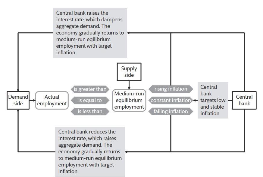
The central bank and a consumer demand shock (Carlin and Soskice 2015)
2.3 Phillips curve
Output affects inflation via the (adaptive expectations) Phillips curve. It shows the output and inflation combinations that the central bank can choose. Inflation will be what is was last year with an adjustment for the output gap or the deviation from NAIRU.
\[\pi_t = \pi_t^E + \alpha(y_t - y_e)\] \[ = \pi_{t-1} + \alpha(y_t - y_e)\]
The Phillips curve can be superimposed on the inflation-output space that contains the central bank loss function. The coefficient \(\alpha\) will determine the slope of the Phillips curve. There are different curves for different levels of inflation expectations. The bliss point is the intersection between the inflation target \((2.0\%)\) and the equilibrium output \((y-e)\). Equilibrium output is the rate of growth of output that does not cause a change in inflation. This is where the economy is at the natural rate of unemployment or NAIRU. The Monetary Rule curve is derived from the tangency of Phillips curves and loss circles.
The Taylor Rule is a way to model central bank decision-making. To move from the MR rule to the Taylor Rule we need to use the IS curve to find the appropriate interest rate. It is the real interest rate \((r)\) that is used to implement policy. The IS curve shows the effect of interest rates on aggregate demand. Remember that this is,
\[y = k(c_0 + a_0 + G) + ka_1 r\]
Or
\[y = A - ar\]
The A term includes the multiplier \((k)\) and all the autonomous elements of aggregate demand such as government spending as well as the autonomous and forward-looking elements of consumption and investment. The three equation models uses the dynamic version of the IS curve so that demand responds to interest rates with a one period lag. Therefore,
\[y_t = A - ar_{t-1}\]
The interest rate that stabilises the economy at the central bank bliss point where inflation and output are at their target is the stabilising rate of interest \((r_s)\). As we have seen above, this can change if there are changes in autonomous spending that require an offset from interest-rate sensitive parts of the economy.
2.4 Forecasting
Central bank forecasting is key to the model. This includes the parameters and the lags in the adjustment process. The central bank has to forecast the PC curve and the IS curve. It has to determine whether the shock is temporary or permanent. If there is uncertainty, the central bank will have to try to steer a middle course.
The Bank of England produces a quarterly inflation report that shows its forecasts for inflation. Here is a visual summary of the report. You can read the full report here.
The main points of the report are
Pay is rising at a faster rate
The UK economy is growing just above its speed limit
Interest rate rises should be gradual and limited…
…and are expected to bring inflation back to 2.0%
The nature of Brexit will affect the UK economy.
2.5 Deflation
Deflation is a major problem that has affected the world economy since the Global Financial Crisis. The Covid-19 Crisis has exacerbated this. This is an example of the way that the deflation trap can be examined in the New Keynesian model. The Fisher equation is
\[i = r + \pi^E\]
As we know, the central bank will adjust the nominal rate in order to change the real rate of interest. This will influence aggregate demand through the Is curve. Due to the zero bound, the minimum real interest rate that can be achieved is the negative of the expected inflation rate.
Figure 3.3 shows the full three equation model for the deflationary zero-bound trap. This shows the process whereby the real interest rate is pushed upwards by deflation and the output gap. There will be no natural return to equilibrium. The central bank cannot adjust real interest rates to stimulate the economy. The central bank loses power.
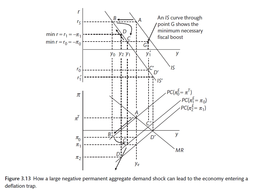
Deflation at the zero-bound(Carlin and Soskice 2015)
The way to deal with this would be: shifting the IS curve (so that the shock is not permanent) with something like a fiscal shock (the MR curve can be replaced with a broader Policy Rule (PR)); create more positive inflation expectations, this could allow the PC curve to shift upwards if it can be achieved; or use quantitative easing to change the behaviour of banks and the IS curve. These are all actions that governments around the world are currently employing in response to the Corvid-19 deflation.
2.6 Supply shocks
A supply shock can come from a shift in the WS curve (caused by changes in union power or unemployment benefits) or from a movement of the PS curve (due to competition or productivity changes). Supply shocks differ from demand shocks in two ways:
- a supply shock will shift the equilibrium level of output;
- a supply shock will shift the MR curve so that it bisects the point to new equilibrium output and the inflation target.
Figure 3.2 shows the adjustment process. The central bank must cut interest rates so that output is above equilibrium raising inflation and wage expectations until the economy moves to the new equilibrium.
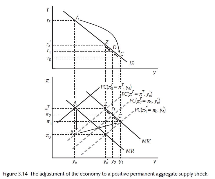
Policy and the supply shock (Carlin and Soskice 2015)