Chapter 3 Expectations
At the end of this chapter you should understand
Why economic agents form expectations
The use of Adaptive Expectations
The Rational Expectations hypothesis
The role of expectations in the New Keynesian model
The Lucas critique

Expectations
The formation of expectation is a key issue in macroeconomics. We have already had forward-looking households and firm making savings and investment decisions as well as central bank forecasting and decision-making.
3.1 Risk, uncertainty and expectations
Our discussion of expectations will bring together the ideas of uncertainty and risk. The distinction between uncertainty and risk is made by (Knight 1921) and (Keynes 1936). Risk can be quantified while uncertainty cannot. Some events have happened before and we have data that can be used to assess probabilities. The risk of death for people with particular age and other characteristics can be assessed for life insurance. However, the probability that an event like the collapse of the Berlin Wall will be seen is less easy to quantify. In the General Theory Keynes argues:
It is safe to say that enterprise which depends on hopes stretching into the future benefits the community as a whole. But individual initiative will only be adequate when reasonable calculation is supplemented and supported by animal spirits, so that the thought of ultimate loss which often overtakes pioneers, as experience undoubtedly tells us and them, is put aside as a healthy man puts aside the expectation of death.
We should not conclude from this that everything depends on waves of irrational psychology. On the contrary, the state of long-term expectation is often steady, and, even when it is not, the other factors exert their compensating effects. We are merely reminding ourselves that human decisions affecting the future, whether personal or political or economic, cannot depend on strict mathematical expectation, since the basis for making such calculations does not exist; and that it is our innate urge to activity which makes the wheels go round, our rational selves choosing between the alternatives as best we are able, calculating where we can, but often falling back for our motive on whim or sentiment or chance.
Keynes is suggesting that people use short-cuts to ease the difficulty of decision-making. Behavioura Economics builds on these ideas with psychological experiments about the ways that expectations are formed and the identification of these short-cuts or heuristics.
3.2 Models of expectations
There are two standard ways that expectations are modelled.
- Adaptive expectations. Expectations are largely based on what has happened in the past.
- Rational expectations. Expectations are based on the module that is being used by the economist.
You will notice that we have been using adaptive expectations for wage setting and price setting but rational expectations for the central bank. In coming chapters we will also suggest that international investors buying and selling foreign exchange are also using rational expectations to make decisions about the future. The rationale for these choices is that central banks and international investors spend a lot of time thinking about the future economy and the future direction of exchange rates, they employ economists and other experts to make predictions; regular people do not think so much about future inflation and have less incentive under normal conditions to get forecasts about inflation correct. These assumptions can, of course, be questioned. These are a simplification that can be justified on some occasions but not others. Rational expectations tend to rule out the development of speculative bubbles that appear to have been an important part of the Global Financial Crisis.
3.3 Phillips curve and expectations
Inflation expectations
\[E(\pi_t | \theta_{t-1}) \equiv \pi_t^E\]
Expected inflation is based on past information. As the agents have all the information up to \(t_1\), this means that only random shocks can bring a surprise to inflation. The Phillips curve will depend on the way that inflation expectations are modelled. The standard curve is
\[\pi_t = \pi_t^E + \alpha(y_t - y_e)\]
What do we know about inflation? Figure 4.2 shows the evolution of inflation. There are different regimes: from 1801 to 1916 inflation was volatility around zero; the 1930s and 40s were more volatile; the 1950s and 60s were positive and the 1970s and 1980s had high inflation; the final period s one of deflation. The 1950s and 1960s can be seen against the backdrop of the 1930s and the Keynesian revolution. Supply-side changes in the 1950s and 1960s means that the underling rate of unemployment increased and the trade off between unemployment and inflation changed: there was a shift in bargaining power towards workers (an upward shift in the WS curve), a fall in productivity caused by an end to the Fordist against in the production line (a downward shift in the PS curve). Figure 4.1 shows this change: the equilibrium output \((y_e)\) level and the Phillips curve (relationship between output and inflation) will change. With adaptive expectations being updated for the last increase in inflation, there can be an upward spiral in inflation.
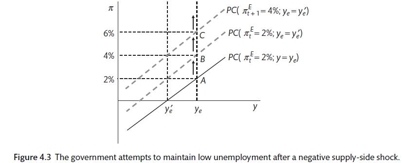
Adaptive expectations and the inflationary spiral (Carlin and Soskice 2015)
(Friedman 1968) and (Phelps 1968) argued that the Phillips curve was vertical in the long-run and that an increase in employment beyond that connected with the natural rate would just cause inflation expectations and inflation to rise. They short-run Phillips curve, they argued, was determined by the level of inflation expectations. There is a discussion of Friedman, Phelps and the evolution of macroeconomic models here
\[\pi_t^E = \pi_{t-1} + \alpha (y_t - y_s)\]
The equation can be re-arranged to show how inflation changes.
\[\pi_t - \pi_{t-1} = \Delta pi = \alpha(y_t - y_e)\]
Therefore the relationship between unemployment and inflation will hold only as long as the government does not try to run the economy above the equilibrium level of output.
The rational expectations framework suggests that agents can learn. They understand the model that is being used. They do not make systematic mistakes. In the rational expectations framework, it is only unsystematic shocks that cause inflation to differ from expectations.
\[\pi_t = \pi_t^E + \alpha(y_t - y_s) + \varepsilon_t\]
Therefore,
\[y_t = y_s - \frac{\varepsilon_t}{\alpha}\]
The difference between adaptive expectations and rational expectations. If the central bank wants to reduce the inflation target in conditions where expectations are formed adaptively, it will increase interest rates to reduce output below the stabilising rate so that inflation expectations are pushed lower. There is an output-employment cost to reducing inflation. If expectations are formed rationally, changing the rate of inflation is more rapid and less painful.
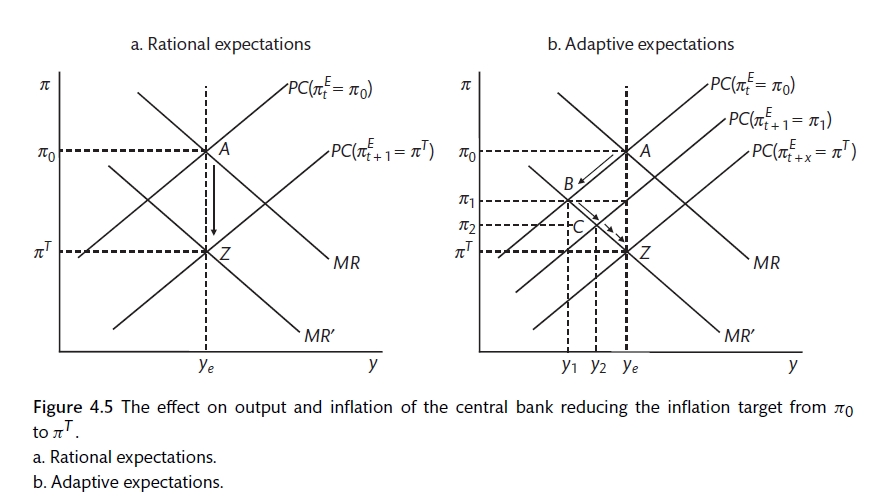
Central bank policy under rational and adaptive expectations (Carlin and Soskice 2015)
With rational expectations, agents believe that inflation will be at the target apart from a random, non-systematic element. In this case, the central bank will keep output at the stabilising rate and agents adjust their inflation expectations to the new target. The three major differences between an economy that is largely working under rational expectations from one where expectation arise adaptively are:
- the economy remains at equilibrium apart from the random shocks;
- there is no inbuilt method for inflationary or deflationary forces to arise;
- the central bank does not have to worry about forecasts and lags;
- since wage-setters and price-setters are forward-looking, the central bank can influence expectations directly.
3.4 Central bank expectations policy
There is a huge amount of central bank effort devoted to managing expectations. If the central bank intentions are known and credible, an inflation shock is a one-period shock that should not change expectations. If inflation expectations are anchored, there is no need for a painful adjustment that involves unemployment. This idea can be captured by modifying the adaptive expectations Phillips curve to incorporate credibility with expectations formed as a weighted sum of the inflation target and lagged inflation. \((\chi)\) determines the weight to credibility.
\[\pi_t = \chi \pi^T + (1 - \chi) \pi_{t-1} + \alpha(y_t - y_s)\]
\[\pi^T_t = \chi \pi^T + (1 - \chi) \pi_{t-1}\]
The two extremes are \(\chi = 1\) where inflation expectations are fully anchored to \(\chi = 0\) where expectations are adaptive. The more credibility that the central bank has the lower the cost of maintaining the target. Two major factors affect credibility: communication and transparency. The communication strategies of the central bank seek to address the questions that may arise: will the central bank stick to the target; can the central bank shape inflation expectations? These factors depend on the independence of the central bank from political pressure, as well as history, culture and other institutions. In addition, the more transparent central bank decision-making and objectives, the less chance of a surprise.
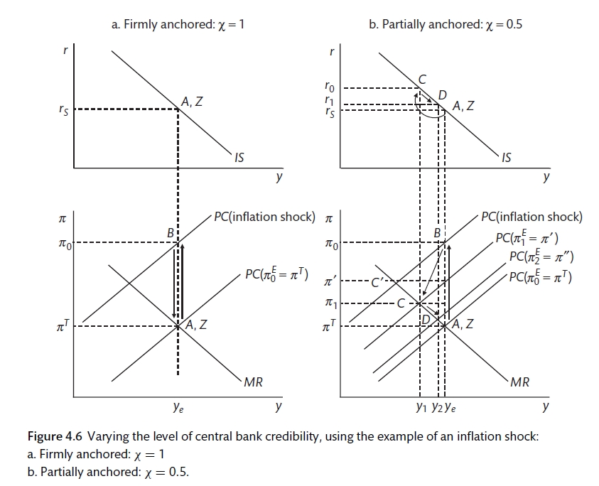
Central bank credibility (Carlin and Soskice 2015)
Therefore, if the central bank has credibility it becomes much easier and less painful (in terms of unemployment) to reduce inflation. For many years it was argued that the credibility of the German central bank (the Bundesbank) was part of the reason for the stability and success of the German economy. The creation of the Euro and the Eurozone was at least partly an attempt to extend this credibility to other European nations. Now it appears that credibility may have gone too far. Most people do not remember inflation. People do not expect inflation to be above 2.0%.
3.5 The Lucas critique
New Classical Economics has developed since the 1970s. This is based on formal microfoundations where agents have forward-looking, model-consistent expectations. Real Business Cycle economics is the result. The Lucas Critique (Lucas 1976) says that economic relationships will change when policy regimes change because economic agents will adapt their behaviour. If agents are set expectations rationally, it is not possible for the government to engineer a one-off increase in output (ahead of an election). Inflation expectations remain anchored. A government controlled central bank would not have the same effect. Now inflation expectations would rise with the increase in government spending and a more painful process would be required to bring it back down. Similarly, if we assume rational expectations, a cut in the inflation target can be made without any pain. Therefore, the use of rational expectations is controversial and at the extreme can suggest that the government has no positive influence over the economy.
#Money, Banking and the Financial Sector At the end of this chapter you should understand
How the financial system is represented in the economy
The central bank lending rate and the policy rate
Credit rationing and information asymmetries
Bank liquidity, solvency and the balance sheet

Bank
This chapter is about the role of money and banking in the macro economy. This subject has been ignored in some macroeconomic models. Models such as the Real Business Cycle assume that the financial system operates smoothly without any frictions. If the system is working well, economic agents can carry out their planned expenditure using money and credit. However, the Global Financial Crisis (GFC) made clear the disruption that may be felt when the financial system is not working well. These disruptions can have major effects on the overall economy and therefore should not be ignored.
There are two new features introduced to the model when we look more closely at the financial system:
There is a distinction between the policy rate and the lending rate;
Banks intermediate between depositors and borrowers and impose borrowing constraints on some parties (credit rationing).
3.6 Banking mark-up
Up to now the central bank has been able to set the interest rate to obtain the level of economic activity that is required. However, it is necessary to distinguish between the bank rate and the lending rate that is set by financial institutions. It is the lending rate that is important for the financial decisions made by economic agents. The lending rate is the mark-up on the policy rate that is determined by the banks’ optimising decisions. For the IS curve, we now have the lending rate on the y-axis and denote the Policy rate as that set by the central bank. The difference between the two is banking mark-up. This allows an analysis of shocks to the banking system that can determine the spread.
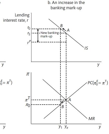
The Banking Mark-up (Carlin and Soskice 2015)
If there is a shock to the banking system unanticipated by the central bank that results in an increase in the margin that banks charge above the policy rate (maybe because they become more concerned about bad loans), this will cause an unanticipated shift along the IS curve and will push the economy below the stabilising level of output. In these cases, the central bank must cut interest rates to reduce the lending rate and bring output back to the stabilising level.
##Money and the macroeconomy Money has three functions:
- Means of transaction. It is used to buy things. There is no need to barter. The more transactions the more money that is required.
- Unit of account. It allows comparison. If the value of money changes rapidly, it is difficult to use for comparison.
- Store of value. It is used for savings. If it loses value it is not useful for saving.
Households select the amount of cash that they want to hold. This will be determined by their desire to purchase goods, repay debts and buy assets. It will also be affected by technology (cash alternatives). Banks decide the amount of reserves that they hold by estimating how much they need for customer requests and for settling balances with other banks. Generally, other assets will yield more than reserves. The liquidity ratio is the ratio of reserves to bank deposits. Therefore, central bank cash is determined by the liquidity ratio, the cash demanded by households and the size of bank deposits. Subject to the liquidity constraint (liquidity rate), commercial banks will create money by making loans when it is profitable to do so. This will depend on the demand for loans, which is set by the IS curve, and the funding costs set by the central bank. Cash is less than 3% of a modern economy. It is assumed that bank deposits do not pay interest and that households can hold either cash, deposits or government bonds. In reality we should also add corporate equity and corporate bonds as potential assets that households could buy.
The commercial bank money is determined by the size of current accounts. Households and firms determine the amount of cash that they will hold. This will be deponent on their income and the level of interest rates. As income increases, households will want to conduct more transactions and will need more money to do that; as interest rates rise, the return on bonds becomes higher and makes bank deposits less attractive.
\[\frac{M^D}{P} = f(y, i, \Phi)\]
Where \(y\) is income, \(i\) is the nominal interest rate and \(/phi\) is the structural changes that take place in the financial sector (such as ATM machines). Given the Fisher equation \((i = r + \pi^E)\), if inflation goes up, this adds to the opportunity cost of holding money and demand for money will fall. These private sector decisions in combination with the policy of the central bank will set the amount of money. \(\Phi\) can also be used to capture things like a change in confidence. In the period after 2008 when there was a loss of confidence in the financial system, the demand for pure cash increased. Fluctuations in the demand for cash as a safe asset mean that the relationship between money and spending is not very stable.
3.7 The financial system
The policy rate is the rate that the central bank lends money to the banking system. If there is payment on reserves, this provides the mechanism that keeps other short-term interest rates close to the policy rate. The reserve rate acts as a floor. It is the lending rate that determines demand in the economy (via the IS rate).
Commercial banks will face a demand for loans and a cost of funds. Commercial banks will borrow from the money market if they do not have sufficient deposits. It is assumed that banks are profit-maximisers. Profits depend on: expected return on loans, cost of funds in the money market and the opportunity cost of bank capital. The expected return will be affected by credit risk (even on secured loans). Bank risk tolerance will vary and the ability of the bank to bear risk will depend on how much capital it has. The spread between the policy rate and the lending rate is determined by risk, risk tolerance and capital. The interest rate margin or banking mark-up equation is
\[r = (1 + \mu^B)r^P\]
\(\mu^B\) is the banking mark-up that depends positively on risk and negatively on risk tolerance and capital.
The policy rate and money market rates are more or less equal in normal conditions. The level of competition in the banking industry will also affect the mark-up of lending rates over policy rates in the medium term. The relatively low level of competition in the UK banking market is believed to make borrowing relatively expensive for UK borrowers with minimal alternatives forms of finance. (Kleimeier and Sander 2017) find that level of competition is the most important, but not the only influence on the extent that central bank interest rate changes are passed through to other interest rates in the economy. There are also debates about the relationship between the level of competition and the stability of the financial system with some suggestions that more competition encourages more risky behaviour.
##Credit constraints Credit rationing is a key feature of the banking system that stems from asymmetric information. This means that households face credit constraints. These credit constrains affect the slope of the IS curve and the power of the multiplier. It is hard for lenders to distinguish between bad luck and moral hazard. The more that borrowers use their own wealth to fund a project, the more confident the bank can be. The lender also has less precise information about future earnings. If a bank charges an average rate, there is a risk of adverse selection. Informational asymmetries mean that assets become very important and that people without assets will find themselves credit constrained. Positive role of banks: maturity transformation; aggregation (bringing together small savings into a usable amount); risk pooling (default is a small part of the total).
3.8 Liquidity risk
Banks face liquidity risk. A bank run is a risk in a fractional banking system. This has encouraged the development of lender of the last resort and deposit insurance. These schemes have to balance providing confidence and preventing moral hazard. Banks also face insolvency risk (asset with less than liabilities). Equity owners, depositor and money-market partners will be affected. Solvency problems can cause liquidity problems as banks become cautious about lending to each other. In the 1930s the Federal Reserve was passive towards banking failure; in 2015 the central bank learnt from the previous mistakes. However, there are limits. In Ireland the debts of the banking system were greater than the resources of the government. The relationship between the government and the central bank was highlighted during the European debt crisis of 2010.