Chapter 6 Growth, Development and Innovation
By the end of this chapter you should understand the following
The causes of growth and the role of capitalism
The connection between the New Keynesian model and long-run growth
Mathematical tools for understanding long-run growth
The Solow model and its augmented versions
Economic convergence: theory and evidence

Cranes
The capitalist explosion of economic growth is a new phenomena. The upswing began around 1750 in the UK. A natural experiment happened with economic planning in the Soviet Union and other countries. It is possible to compare the perforamnce of market-based and command economies. Though the command economies of the Soviet Union and Eastern European nations industrialised quickly and converged towards developed countries, this convergence soon ended and the improvement in per capital GDP stalled. It is argued that in a system without private property, there there is no incentive to innovate or create new products. After the collapse of the ‘communisted’ regimes, the switch from planning to capitalism was painful, showing institutions and history are important. Planning was useful for initial development but not for the later stages. There are three broad explanation for what causes different regions to develop at different rates: geography, culture and institutions.
Assessing the long-run growth performance is the equivalent of saying that we are studying the rate of change of the equilibrium or potential level of GDP. We are assuming that all savings are automatically invested so that we can abstract from the fluctuations. Savings have different effect in different models. In the short-run there is a paradox of thrift; in the medium term the economy returns to equilibrium after increased savings because the central bank cuts interest rates in response to the risk that inflation will fall.
## The long rund and the short run
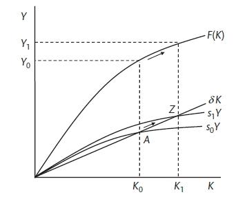
At the heart of the Solow model is a production function with diminishing returns to capital. The shape of the production function \(F(K)\) is concave. There is depreciation that requires some savings to replace the depreciated capital \((\delta K)\). The savings rate (between 0 and 1) means that the effect of savings is the same shape as the production function. If there is an increase in savings, this will add to the capital stock, increase labour productivity and increase output. Once the economy gets back to the point where savings equal depreciation, there is no further increase in the capital stock or the economy. This can be linked to the three equation model because the increase in savings will temporarily leave the economy below is potential. The central bank can cut interest rates to encourage investment. The slope of the production function is the marginal product of capital as it shows the change in output for a change in capital. The marginal product is equal to the real interest rate plus the rate of depreciation. This is consistent with the lower interest rate that the central bank sets.
\[r_z = \delta = MPK_z\]
Investment rises in response to the rate cut and the economy moves to a new equilibrium at higher output and more capital intense method of production.
6.1 The Solow growth model
The Solow-Swan model was an extension of the Harrod-Domar model. It predicts that economies converge to their steady state in the long run and that permanent growth is only achieved by technological progress. Assuming no growth in labour or technological progress, eventually the last capital will only be sufficient to cover depreciation. At that point the economy will cease to grow. If the labour force grows, the economy converges to a steady start of growth where GDP per capital is constant. If there is technological progress, the per-capital growth will be equal to the rate of technological progress.
Swan-Solow model (Carlin and Soskice 2015)
Effective labour AL with A as labour-augmenting tecThe production function for a one-good economy (corn or something else that can be consumed or used for investment) with
\[Y = AF(KN)\]
where production is smooth and continuous and the marginal rates are positive and diminishing. All variables are real. There are constant returns to scale and the Cobb-Douglas function is used,
\[Y = AK^\alpha N^{1-\alpha}\]
In the intensive form where \(K/N = k\) and \(A/K = a\)
\[y = ak\]
A is total factor productivity and \(\alpha\) is capital share of income. Labour share of income is \(1 - \alpha\). Therefore, output per worker will depend on capital per worker and total factor productivity. A will capture the technology, the efficiency with which technology and capital are used and the management quality. This function is concave, reflecting diminishing returns to capital. The average product of capital \(y/k\) is a line from the origin and the marginal product of capital is the slope of the function or
\[MPK = \frac{d(Ak^\alpha)}{dk} = Aak^{\alpha-1}\]
If the labour force grows at a constant rate n and we work in continuous time,
\[n = \frac{\dot{N}}{N} = \frac{dN/dt}{N}\]
Therefore in the future the level of the labour force is
\[N_t = N_0 exp(nt)\]
The capital stock grows at the rate of investment less the depreciation
\[\dot{K} = I - \delta K\]
In a closed economy with no government,
\[S = sY \]
with s as the savings rate
\[\dot{K} = I - \delta K = sY - \delta K = sAK^\alpha N^{1-\alpha} - \delta K\]
Divide through by K to get the growth rate of capital stock
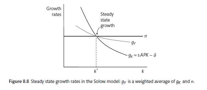
\[g_K = \frac{\dot{K}}{K} = s\frac{Y}{K} - \delta = s APK - \delta\]
Stead growth is when output and capital grow at the same pace so that output to capital ratio must be stable. In a model without technological progress they must grow at the pace of labour.
\[g_Y = g_K = n\]
The capital-labour ratio \((k^*)\) and the capital-output ratio \((V^*)\) will be constant The steady-state requires
\[g_K = s \frac{Y}{K} - \delta = n\]
which implies
\[v^* = \frac{K}{Y}^* = \frac{k}{y}^* = \frac{s}{n + \delta} \]
This is the Harrod-Domar formula. Where the steady state is determined by exogenous variables and does not depend on the production function.
In the steady state: Output and capital grow at the same rate as the exogenously given rate of labour growth. The capital-output ratio is higher the higher the savings rate and the lower the labour growth rate and depreciation.
Swan-Solow Steady State (Carlin and Soskice 2015)
Figure 8.2 shows the steady state where the growth rates of capital, labour and output are equal. This can tell us about the growth of output whereas the more standard Solow diagram in 8.1 shows the growth of output per capita.
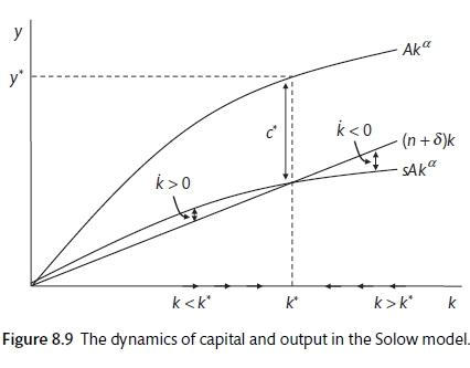
\[k = sAk^{\alpha} - (n - \delta)k\]
The first term tell us how investment is adding to capital per worker, the second term tells us how much investment is required to offset depreciation and the need to equip new workers. Has depreciation risen? In the diagram, \((n +\delta)k\) is a straight line and \(sAK^\alpha\) is the same shape as the production function. Unless the two coincide, capital per work is rising or falling. Where they meet there is equilibrium and with growth in capital per worker and no growth in output per worker. Consumption per worker will also be in a steady state as it is that fraction of output that is not saved.
\[c^* = A(k^*)^\alpha - sA(k^*)^\alpha = (1 - s)A(k^*)^\alpha\]
The equilibrium quality \(K^* = 0\) implies that
\[k^* = \left ( \frac{As}{\delta + n} \right )^{\frac{\alpha}{1 - \alpha}}\]
steady state capital ratio
\[y^* = A(k^*)^\alpha = A^{\frac{1}{1 - \alpha}} = \left ( \frac{s}{\delta + n} \right ) ^{\frac{\alpha}{1 - \alpha}}\]
Savings and growth (Carlin and Soskice 2015)
With the Solow model, the higher the savings the higher the level of GDP. However, consumption is a better measure of welfare (see China and the calls for more consumption). The level of savings that will maximise consumption is called ‘The Golden Rule savings rate’. Figure 8.11 shows that consumption is maximised at the Golden Rule savings rate consistent with \(k_GR^*\) which is tangential to the production function with the same slope as \((n + \delta)k\). With competitive markets the slope of the production function, which is the marginal product of capital, has the slope of \(r + \delta\). The marginal product of capital has to cover the rental cost plus depreciation. Consumption is maximised when \(r + \delta = n + \delta\). So \(r = n\). Total savings equal total profits and total wages are equal to total consumption. Therefore, with a Cobb Douglas production function, the savings rate is equal to \(\alpha\) or capital’s share of output.
A shock to the savings rate (a move to more normal levels in China) would lead to a shift backwards down the production function and a fall in the stable rate of capital per worker but no change in the growth rates (which remain at n).
Using the steady state of output per person,
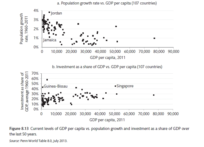
\[y^* =\left ( \frac{s}{\delta + n} \right )^{\frac{\alpha}{1 - \alpha}}\]
suggests that output per capital will rise with total factor productivity (A), rise with the savings (investment) rate and fall with population growth. However, cross country evidence from the Penn Tables suggests that the relationship is flimsy. ASIDE: use this as an exercise. It is clear that the model cannot explain the large divergence in output per capita. There is something more.
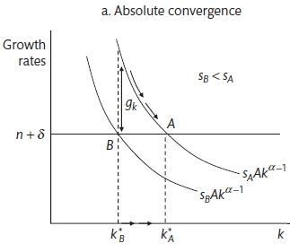
To look at convergence we will distinguish between absolute convergence and relative convergence. From the fundamental Solow Law of Motion,
\[\dot{k} = sAk^\alpha - (n + \delta)k\]
divide through by k to get the growth of the capital labour ratio
\[g_k = sAK^{\alpha - 1} - (n + \delta)\]
The balance growth path for a rich and a poor country will differ only in the savings rate. The poor country has a lower capital-labour ratio and therefore lower output per capita. In the steady state each country is growing such that
\[g_K = g_Y = n\]
and
\[g_k = g_y = 0\]
In the Solow model, an increase in savings will lead to an increase in the capital-labour ratio and due to the diminishing marginal returns, this will increase output per capita. However, there is little evidence that absolute convergence has happened systematically.
6.2 Convergence
The basic Swan-Solow model suggests that countries should converge towards the same level of economic activity. If there is low output and capital per person, the relatively high prodcutvity of capital should attract investment, capital deepening and high levels of economic growth. Meanwhile, countries with relatively high capital per person will gowth more slowly. There is a **testable hypothesis* that growth of countries with low per-capital GDP should be higher than that of countries with high per-capital GDP. There is mixed evidence.
Convergence (Carlin and Soskice 2015)
Conditional convergence suggests that countries of similar GDP per capital will tend to converge. This means that rich and poor have different production functions. There is much more evidence in favour of conditional convergence. Figure 8.15b shows the convergence of the OECD countries in the Golden Age of 1950 to 1973. (Mankiw, Romer, and Weil 1992) test this across a broader range of countries and find evidence of convergence but at a slower pace than would be expected by by theory.
###Human capital One factor that could explain different production functions is a resource that is more productive in some countries than others. Figure 8.16 shows that there is a positive relationship between educational attainment and GDP per capita - though this does not tell us anything about causation. The production function can be amended to include h for the quality of human capital
\[Y = AK^\alpha (hN)^{1 - \alpha}\]
The steady state output per head is now the same as before but A is replaced with \(h^{1 - /alpha}A\)
(Mankiw, Romer, and Weil 1992) test a version of this model and find that it provides a much better explanation for the differences in countries. They find strong evidence for conditional convergence.
Conditional convergence (Carlin and Soskice 2015)
###Technological progress US growth in output per person has been in the region of 2.5% since 1870. The Solow growth model does not pin down technological progress but it shows the way that progress must evolve to be consistent with balanced or steady growth. In this form technological progress must not use up any resources in the economy (because these are used for capital accumulation and depreciation) and must be used to enhance labour productivity. This is called Harrod-neutral or labour-augmenting technological progress. It is usually described as a steady process that increases output per worker by a particular percentage (x) per year. The Cobb-Douglas function becomes
\[Y = K^\alpha(A N)^{1 - \alpha}\]
where \(A_t = A_0 exp(xt)\)
A now changes from Total Factor Productivity that can affect the level of output to an exponential process that represents a movement in the technological frontier over time. In this case,
\[g_Y = g_K = n + x\]
\[g_y = g_k = x\]
Define efficiency units as \(\tilde{L} = AL\)
\[\tilde{y} = \frac{Y}{A_tN} = \frac{y}{N}\]
\[\tilde{K} = \frac{K}{A_t N} = \frac{k}{N}\]
The fundamental law of motion becomes
\[\tilde{k} = s(k)^\alpha - (n + \delta + x)k\]
and setting this to zero gives the steady state
\[s(k)^\alpha = (n + \delta + x)k\]
\[\tilde{y}^* = \tilde{k}^* = \left ( \frac{s}{a + \delta + x} \right )^{\frac{\alpha}{1 - \alpha}}\]
Therefore the steady state level of output per worker is
\[y_t^* = A \tilde{k}^* = \left ( \frac{s}{a + \delta + x} \right )^{\frac{\alpha}{1 - \alpha}}\]
This shows that output per capital is increasing in technological progress and savings and declining with population growth and the rate of depreciation. Economies with lower fertility and more technological process will have higher GDP per capita. Figure 8.7 shows the Solow production function with exogenous technological progress. This is very similar to the standard model but it is in efficiency units. The line \(n + \delta + x\) shows the investment that is required to maintain the efficiency level of capital per worker. Therefore an increase in technological process will require more investment and will increase output per capita and will raise the equilibrium level of capital per worker.
##Growth accounting Solow’s method of accounting for total factor productivity is called growth accounting. It covers the intangible aspects of human progress. Start with the standard Cobb-Douglas
\[Y = AK^\alpha N^{1-\alpha}\]
take logs and differentiate with respect to time,.
\[y_Y = g_{TFP} + \alpha g_K + (1 - \alpha)n\]
This can be re-arranged to
\[g_{TFP} = (g_Y - n) - ag_k + an = g_y + ag_k\]
so
\[g_y = \alpha g_k + g_{TFP}\]
6.3 Endogenous Growth
The Solow model has long run growth deponent on the exogenous increase in TFP. Romer identified some endogenous features that could overcome diminishing returns to capital. These could include knowledge spillovers from accumulation of physical capital, investment in research and development or in human capital. In the Solow model innovation is an exogenous public good that is non-excludable. There are no costs to innovation. The endogenous growth literature sees innovation as an investment that will realise temporary rents as others take time to adapt. Endogenous growth has a factor (capital, human capital or ideas) that have constant rather than diminishing returns. Figure 8.18 shows a production function with constant returns to capital. Now the lines are straight rather than concave and there is a steady state where the investment \((sY)\) is just equal to the depreciation and the increase in the population. If savings increase, the accumulation of capital increase without limit. Now we distinguish between those working in production \((N^Y)\) using capital and blueprints into final goods and those working in research \((N^R)\) creating new blueprints. We can re-draw the production function
\[Y_t = K_t^\alpha(A_tN_t^Y)^{1 - \alpha}\]
Where \(A_t\) is not the blueprints rather than exogenous technological progress. With \(N = N^Y + N^R\), the source of endogenous growth is the constant returns to the accumulation of blueprints.
\[A_t = cA^\eta N_t^R\]
A will accumulate in proportion (c) to the accumulation of ideas. \(\eta\) is the key variable. If it is above 1 there are spillovers from the accumulation of blueprints and if it is one there are constant returns. This is called the Romer model (P. M. Romer 1990).
When \(\eta = 1\) we have
\[A_t = cA_tN_t^R\]
Divide by A to get the growth rate of ideas.
\[g_A = cN_t^R\]
With \(\eta = 1\), there is a steady state of endogenous growth. Now the steady state growth rate is higher the more people are employed in research.
6.4 Schumpeterian growth: the Aghion-Howitt model
Creative destruction is the creation of temporary innovation rents with new processes, new products or new ways or organising the factors of production. Old processes and product as destroyed as a result. The advantage is maintained by patents, trade secrete and first-mover advantage. The whole process depends on there being a place for new firms to develop, an ability to overcome existing firms and institutions that ensure that entrepreneurs are able to take advantage of their luck or skill.
The Solow model can be linked to the Schumpeterian model by focusing on factor accumulation and technological progress. Using the Solow model we can assess the way that changes in the rate of technological progress \((x)\) will affect other variables. All else equal, a higher level of technological progress will mean lower level of capital per efficiency unit of labour \((\tilde{g_k}).\) Seen Figure 8.17. This is shown on Figure 8.19. This is called the Solow Steady State Relationship. A swifter rate of exogenous technical progress requires less capital per person (as more output is achieved with the same amount of capital) and shifts the economy to a faster pace of growth with lower capital intensity (for the given savings). A Schumpeterian relationship were there is more innovation when there is higher capital (and output) per efficiency unit of labour. This is added to Figure 8.19 to create an equilibrium between the rate of technological progress and the steady state of capital per efficiency unit of labour.
How can this be used to create higher steady state growth? Either an increase in savings (and investment) or an increase in the returns to innovation. Tax could be used to increase savings and investment and thereby shift the Solow relationship upwards; similarly taxes and subsidies could be used to stimulate innovation. ASIDE: there are many other policies. Therefore, a (tax induced) increase in savings will lead to more capital and a higher level of economic growth rate. There is a shift in the Solow relationship and also a move up the Schumpeterian relationship. In this case a regression test of the effect of investment on the output as there is a secondary effect (shown by the move up the Schumpeterian curve) as the larger economy provides a greater incentive to innovate. There is an endogeneity issue here. Alternatively there may be policy to increase the level of R&D will shift the Schumeterian relationship upwards,
Aghion and Howitt model innovation and new higher quality products. It is suggested that too much competition can stifle innovation as there is less change to take advantage. However, Schumpeter also stressed the importance of competition in spurring innovation. This suggests a inverse=U shaped relationship between competition and innovation. The details of the model suggest that there are three sectors: at the technological frontier the return from innovation are really high, here more innovation boosts innovation; just behind the innovation frontier, the scope for innovation is less and more competition means less innovation as it is unlikely that this will allow sufficient scope to escape the monopoly pricing; at the lowest level there is no inventive to innovate but there is automatic spill-over from the other sector. Aghion find an inverse-U shaped relationship between the cost-price spread and the level of patents (Aghion et al. 2005). Another study (Aghion et al. 2009) suggests that increased competition (from overseas companies in this case) will increase patents at frontier firms but will decrease innovation amongst firms just below the innovation frontier.
The Schumpeterian model also emphasises the link between business fluctuations and long-term investment. There seems to be a link between business fluctuations and innovation. Some evidence suggests that 20% of innovation is about the entrance of new firm to the market. Other studies suggest that the entrenchment of existing firms in the planned economy system was one reason for the lack of innovation and dynamism. There is also an additional argument in favour of intervention to stabilise the economy: credit constraints in the downturn can reduce the amount of innovation inducing R&D. ASIDE: there is some evidence of this from recent assessment of the port-GFC productivity slowdown in developed economies.