Chapter 6 Flow & Control
In this chapter we will study the importance of flow and control in computer programming. Most of the information of this chapter is from base R functionality, but as usual, we will leverage some parts of the tivdyverse.
Dr. Sonderegger’s Video Companion: Video Lecture.
6.1 Control and Flow
Often it is necessary to write scripts that perform different action depending on the data or to automate a task that must be repeated many times. To address these issues we will introduce the if statement and its closely related cousin ifelse. To address repeated tasks we will define two types of loops, a while loop and a for loop.
Although control may not immediately seem important in code, the uses for it become exponentially more important as the complexity of code grows. Control allows an individual to quickly turn on and off features of a function, easily run immense amounts of code with minimal syntax, provide improved functionality by catching errors before they occur, and so many other elements we are slowing growing into throughout this book. Control is the building block to make code that is functional, easy-to-use, and free of erroneous components that may otherwise cause users to struggle to get the desired output.
6.2 Logical Expressions
The most common logical expressions are the numerical expressions you have study in a mathematics course and include <, <=, ==, !=, >=, >. These are the usual logical comparisons from mathematics, with != being the not equal comparison. For any logical value or vector of values, the ! flips the logical values.
##   A B
## 1 1 6
## 2 2 5
## 3 3 4
## 4 4 3
## 5 5 2
## 6 6 1## A B A==3? A!=3? A<=3?
## 1 1 6 FALSE TRUE TRUE
## 2 2 5 FALSE TRUE TRUE
## 3 3 4 TRUE FALSE TRUE
## 4 4 3 FALSE TRUE FALSE
## 5 5 2 FALSE TRUE FALSE
## 6 6 1 FALSE TRUE FALSEIf we have two (or more) vectors of logical values, we can do two pairwise operations. The “and” operator & will result in a TRUE value if all elements are TRUE. The “or” operator | will result in a TRUE value if any elements are TRUE.
df %>% mutate(C = A>=5,  D = B<=4) %>%
  mutate( result1_and = C & D,  #    C and D both true
          result2_or = C | D)   #    C or D true
## A B C D result1_and result2_or
## 1 1 6 FALSE FALSE FALSE FALSE
## 2 2 5 FALSE FALSE FALSE FALSE
## 3 3 4 FALSE TRUE FALSE TRUE
## 4 4 3 FALSE TRUE FALSE TRUE
## 5 5 2 TRUE TRUE TRUE TRUE
## 6 6 1 TRUE TRUE TRUE TRUENext we can summarize a vector of logical values using any(), all(), and which(). any() looks for at least one TRUE, all() requires all elements to be TRUE, which() provides the location of the TRUE elements.
## [1] TRUE## [1] FALSE## [1] 1 2Finally, we often need to figure out if a character string is in some set of values. Here we create a small data frame with a letter index (maybe a indicator or categorical group variable) and assign a random value to each. We can then use the operator %in% to search through the vector Type and return all elements that match elements within our search vector (here we are searching for the A and B categories).
##   Type       Value
## 1    A  0.59402990
## 2    B  0.05041084
## 3    C  0.61352322
## 4    D  0.37585796
## 5    A  1.59620506
## 6    B -1.15972350
## 7    C  0.52400185
## 8    D -0.47470014
# df %>% filter( Type == 'A' | Type == 'B' )
df %>% filter( Type %in% c('A','B') ) # Only rows with Type == 'A' or Type =='B'## Type Value
## 1 A 0.59402990
## 2 B 0.05041084
## 3 A 1.59620506
## 4 B -1.159723506.3 Decision statements
6.3.1 Simplified dplyr wrangling
A very common task within a data wrangling pipeline is to create a new column that recodes information in another column. Consider the following data frame that has name, gender, and political party affiliation of six individuals. In this example, we’ve coded male/female as 1/0 and political party as 1,2,3 for democratic, republican, and independent. These codings are not very readable, but this is a common way data is stored, often with a ‘key’ that informs the user what the number codings mean.
people <- data.frame(
  name = c('Barack','Michelle', 'George', 'Laura', 'Bernie', 'Deborah'),
  gender = c(1,0,1,0,1,0),
  party = c(1,1,2,2,3,3)
)
people
## name gender party
## 1 Barack 1 1
## 2 Michelle 0 1
## 3 George 1 2
## 4 Laura 0 2
## 5 Bernie 1 3
## 6 Deborah 0 3The command ifelse() works quite well within a dplyr::mutate() command and it responds correctly to vectors. We used this briefly in Chapter 4 without much discussion, but are now ready to use this as an important tool to improve the readability of our variable levels. The syntax is ifelse( logical.expression, TrueValue, FalseValue ). The return object of this function is a vector that is appropriately made up of the TRUE and FALSE results. We will see some tricks of this function as we work through the chapter and exercises.
For example, lets take the column gender and for each row test to see if the value is 0. If it is, the resulting element is Female otherwise it is Male.
##       name gender party gender2
## 1   Barack      1     1    Male
## 2 Michelle      0     1  Female
## 3   George      1     2    Male
## 4    Laura      0     2  Female
## 5   Bernie      1     3    Male
## 6  Deborah      0     3  Female
To do something similar for the case where we have 3 or more categories, we could use the ifelse() command repeatedly to address each category level separately. However, because the ifelse() command is limited to just two cases, we may have to use it many times, keep track to properly not override previous iterations. In these cases, it is better to use a generalization of the ifelse() function that operates on multiple categories. The dplyr::case_when function is that generalization. The syntax is case_when( logicalExpression1~Value1, logicalExpression2~Value2, ... ). We can have as many LogicalExpression ~ Value pairs as we want. As a note, I often find myself using this when recoding large data sets that contain, for example, many different patient diseases that come with simple codings. When I prepare graphs, I want the proper full names showing, and not just a simple code that may not be obvious to all readers. The case_when() function allows me to accomplish this, and I think of it as a ‘mapping’ that takes many different simple codes and outputs a vector with proper disease names. Below we use the case_when() function to deal with renaming the three political parties.
people <- people %>%
  mutate( party2 = case_when( party == 1 ~ 'Democratic',
                              party == 2 ~ 'Republican',
                              party == 3 ~ 'Independent',
                              TRUE       ~ 'None Stated' ) )
people
## name gender party gender2 party2
## 1 Barack 1 1 Male Democratic
## 2 Michelle 0 1 Female Democratic
## 3 George 1 2 Male Republican
## 4 Laura 0 2 Female Republican
## 5 Bernie 1 3 Male Independent
## 6 Deborah 0 3 Female IndependentOften the last case is a catch all where the logical expression will ALWAYS evaluate to TRUE and this is the value for all other inputs that weren’t properly managed previously. As another alternative to the problem of recoding factor levels, we could use the command forcats::fct_recode() function. Chapter 7 - Factors provides more details about this function, but it operates similarly to the dplyr:case_when(), but specifically for data of the factor type.
6.3.2 Base if else statements
While programming, I often need to perform expressions that are more complicated than what the ifelse() command can do. Remember, the ifelse() command only can produce a vector. For any logic that is more complicated than simply producing an output vector, we’ll need a more flexible approach. The downside is that it is slightly more complicated to use and does not automatically handle vector inputs. The upside is that we can produce long chains of if then else statements, provide significant control over the output.
The general format of an if or an if else is presented below:.
# Simplest version
if( logical.test ){ # The logical test must be a SINGLE TRUE/FALSE value
  expression        # The expression could be many lines of code
}

# Including the optional else
if( logical.test ){
  expression
}else{
  expression
}
The else portion is optional and allows you to control what happens if the logical.test returns FALSE. In some cases you might want nothing to happen, in which case no else statement is required. In other cases, you may want to continue exploring possible options or execute a different unique code chunk. The else statement can even be another if command, requiring further logicals to be evaluated prior to output!
Suppose that I have a piece of code that generates a single random variable from the Binomial distribution. This can be thought of as a flipping a coin (a fair coin if we set p = 0.5). We would like to label it head or tails instead of one or zero.
If the logical.test expression inside the if() is evaluates to TRUE, then the subsequent statement is executed. If the logical.test evaluates instead to FALSE, the next statement is skipped. The way the R language is defined, only the first statement after the if() is executed depending on the logical.test. If we want multiple statements to be executed (or skipped), we will wrap those expressions in curly brackets { }. I find it easier to follow the if else logic when I see the curly brackets so I use them even when there is only one expression to be executed (they are not strictly required, so sometimes I get lazy if the resulting expression is a single line of code). Also notice that the RStudio editor indents the code that might be skipped to try help give you a hint that it will be conditionally evaluated.
## [1] 1# convert the 0/1 to Tail/Head
if( result == 0 ){
result <- 'Tail'
print("Output from the if() statement, this means we saw a Tail! ")
}else{
result <- 'Head'
print("Output ffrom the else() statement, this means we saw a Head!")
}## [1] "Output ffrom the else() statement, this means we saw a Head!"## [1] "Head"Try running the code chunk above many times - the output in the textbook will be completely random if it is showing heads or tails! Notice as you run the code chunk over and over that in the Environment tab in RStudio (default location is the upper right corner), the value of the variable result changes as you execute the code repeatedly.
To provide a more statistically interesting example of when we might use an if else statement, consider the calculation of a p-value in a 1-sample t-test with a two-sided alternative. If you are unfamiliar with this calculation, the area is found based on the ‘sign’ (positive/negative) of the corresponding test statistic. The calculation can be summarized as:
If the test statistic t is negative, then p-value = \(2*P\left(T_{df} \le t \right)\)
If the test statistic t is positive, then p-value = \(2*P\left(T_{df} \ge t \right)\).
Below provides code that executes the proper calculation by checking the sign of the test statistic (t). You again may want to run this code chunk many times and watch what changes as the value of t changes! You’ll notice that t jumps around the value of zero randomly, being positive or negative with roughly \(50\%\) probability, yet the p-value is properly calculated each time! The larger the magnitude of t (that is, the absolute value of t), the smaller the corresponding p-value.
# create some fake data
n  <- 20   # suppose this had a sample size of 20
x  <- rnorm(n, mean=2, sd=1)

# testing H0: mu = 0  vs Ha: mu =/= 0
t  <- ( mean(x) - 2 ) / ( sd(x)/sqrt(n) )
df <- n-1
if( t < 0 ){
  p.value <- 2 * pt(t, df)
}else{
  p.value <- 2 * (1 - pt(t, df))
}

# print the resulting p-value
p.value
## [1] 0.9490959This sort of logic is necessary for the calculation of p-values and something similar is found somewhere inside the t.test() function.
6.3.3 Nested if else statements
Finally we can nest if else statements together to allow you to write code that has many different execution routes. The example below random generates a number between 0 and 5 and then strictly rounds UP (this is known as the ceiling()). Depending on the number drawn, the output changes! Again - try it many times to see how ti works, and see how the value of rand.numb changes in the Environment tab of RStudio.
# randomly grab a number between [0,5] and round it up to 1,2,3,4,5
rand.numb <- ceiling( runif(1,0,5) )
if( rand.numb == 1 ){
  print('We got a 1!')
}else if( rand.numb == 2 ){
  print('A 2 was observed!')
}else if( rand.numb == 3 ){
  print('The number 3 was drawn!')
}else{
  print('This was either a 4 or 5, not quite sure!')
}
## [1] "A 2 was observed!"6.4 Loops
It is often desirable to write code that does the same thing over and over, relieving you of the burden of repetitive tasks. To do this we’ll need a way to tell the computer to repeat some section of code over and over. However, we’ll more then likely want something small to change each time through the loop. Loops give us a way to execute the same code many times, changing something slightly each ‘iteration’ of the loop, and provide the computer either how many times to run the loop or a condition for when to stop repeating.
6.4.1 while Loops
The basic form of a while loop is as follows:
# while loop with multiple lines to be repeated
while( logical.test ){
  expression1      # you can have as much code here as necessary!
  expression2
}
Be warned now that while loops require that the conditions within the logical.test are updated within the loop, in the above this is include as something like expression2 changing the value within the logical.test. If this doesn’t happen, then welcome to the world of infinite looping, something we would like to avoid!
The computer will first evaluate the test expression logical.test. If it is TRUE, it will execute the code within the while loop, denoted above as expression1 and expression2. When the code within the loop is completed, evaluation returns to the beginning of the while loop and evaluates the logical.test again. If it is still TRUE, the loop will execute again. This continues until the logical.test finally evaluates as FALSE. Hence the warning above. Below is a little code chunk that doubles the value of x each iteration, and eventually x becomes \(100\) or greater, and the loop stops. If you run the code chunk below, notice that the final value of x is set to \(128\), which fails the condition x < 100.
x <- 1
while( x < 100 ){
  print( paste("In loop and x is now:", x) )  # print out current value of x
  x <- 2*x
}
## [1] "In loop and x is now: 1"
## [1] "In loop and x is now: 2"
## [1] "In loop and x is now: 4"
## [1] "In loop and x is now: 8"
## [1] "In loop and x is now: 16"
## [1] "In loop and x is now: 32"
## [1] "In loop and x is now: 64"It is very common to forget to update the variable used in the test expression. In that case the test expression will never be FALSE and the computer will never stop. This unfortunate situation is called an infinite loop. Avoid ever letting this happen - you have now been warned twice!
6.4.2 for Loops
Often we know ahead of time exactly how many times we should go through the loop or can control the numbers of times based on the values within a vector of interest. We could use a while loop, but there more specific construct called a for loop that is useful for execution of code a known number of times.
The format of a for loop is as follows:
The index variable will take on each value in vector in succession and the next statement will be evaluated. As always, the statement can be multiple statements wrapped in curly brackets {} and include as much code as necessary to get the job done. Notice how the statement below changes as the for loop is executed.
## [1] "In the loop and current value is i = 1"
## [1] "In the loop and current value is i = 2"
## [1] "In the loop and current value is i = 3"
## [1] "In the loop and current value is i = 4"
## [1] "In the loop and current value is i = 5"
What is happening is that i starts out as the first element of the vector c(1,2,3,4,5), in this case, i starts out as 1. After i is assigned, the statements in the curly brackets are then evaluated. Once all code within those statements is executed , i is reassigned to the next element of the vector. This process is repeated until i has been assigned to each
element of the given vector. Although traditionally we use i and j and the index variable, R is a flexible language that will allow you to use any object as your iterator.
While the recipe above is the minimal definition of a for loop, there is often a bit more set up to create a result vector or data frame that will store the steps of the for loop. We don’t typically want to print text to the screen, but store the output of a calculation into an object for later use. The code below shows an outline of how we might create a result object that will contain the output of our code.
N <- 10
result <- NULL     # Make a place to store each step of the for loop
for( i in 1:N ){
  # Perhaps some code that calculates something
  result[i] <-  # something
}
We can use this loop to calculate the first \(10\) elements of the Fibonacci sequence. Recall that the Fibonacci sequence is defined by \(F_{i}=F_{i-1}+F_{i-2}\) with two starting conditions \(F_{1}=0\) and \(F_{2}=1\). Although for clarity of the book the object F is output to screen with the print() function, notice by running the code in your own terminal, you will end up with an F object that stores the first \(10\) Fibonacci numbers.
N <- 10                # How many Fibonacci numbers to create
F <- rep(0,2)         # initialize a vector of zeros
F[1] <- 0              # F[1]  should be zero
F[2] <- 1              # F[2]  should be 1
print(F)               # Show the value of F before the loop
## [1] 0 1for( i in 3:N ){
F[i] <- F[i-1] + F[i-2] # define based on the prior two values
print(F) # show F at each step of the loop
}## [1] 0 1 1
## [1] 0 1 1 2
## [1] 0 1 1 2 3
## [1] 0 1 1 2 3 5
## [1] 0 1 1 2 3 5 8
## [1] 0 1 1 2 3 5 8 13
## [1] 0 1 1 2 3 5 8 13 21
## [1] 0 1 1 2 3 5 8 13 21 34For a more statistical case where we might want to perform a loop, we can consider the creation of the bootstrap estimate of a sampling distribution. The bootstrap distribution is created by repeatedly re-sampling with replacement from our original sample data, running the analysis for each re-sample, and then saving the statistic of interest. This is a very powerful statistical technique that I hope everyone gets to learn in a later course! Here is some code that runs a bootstrap analysis of the mean Height from the trees data set.
library(dplyr)
library(ggplot2)

# bootstrap 5000 resamples from the trees data set.
SampDist <- data.frame(xbar=NULL) # Make a data frame to store the means
for(i in 1:5000){
  ## Do some stuff
  boot.data <- trees %>% dplyr::sample_frac(replace=TRUE)
  boot.stat <- boot.data %>% dplyr::summarise(xbar=mean(Height)) # 1x1 data frame

  ## Save the result as a new row in the output data frame
  SampDist <- rbind( SampDist, boot.stat )
}

# Check out the structure of the result
str(SampDist)
## 'data.frame': 5000 obs. of 1 variable:
## $ xbar: num 77.5 77.5 76 74.1 73.8 ...# Plot the output
ggplot(SampDist, aes(x=xbar)) +
geom_histogram( bins = 25, color='black', fill='grey50') +
labs(title='Trees Data: Bootstrap distribution of Mean Height (xbar)')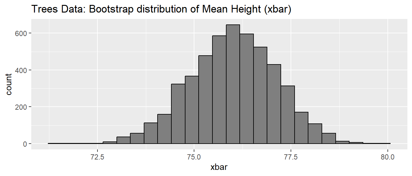
6.5 Functions
It is very important to be able to define a piece of programming logic that is repeated often. For example, I don’t want to have to always program the mathematical code for calculating the sample variance of a vector of data. Instead I just want to call a function that does everything for me and I don’t have to worry about the details.
While hiding the computational details is nice, fundamentally writing functions allows us to think about our problems at a higher layer of abstraction. For example, most scientists just want to run a t-test on their data and get the appropriate p-value; they want to focus on their problem and not how to conduct the calculation in detail. Another statistical example where functions are important is a bootstrap data analysis where we need to define a function that calculates whatever statistic the research cares about.
The format for defining your own function is
function.name <- function(arg1, arg2, arg3){
  statement1 # likely involving arg1, arg2, and/or arg3
  statement2 # likely involving arg1, arg2, and/or arg3
}
where arg1, arg2, and arg3 are the arguments of the function in which the user can change based on their needs. To illustrate how to define your own function, we will define a variance calculating function. The function takes in a vector of values x, which can be of any size and contain any variety of numbers, and outputs the properly calculated sample variance.
# define my function
my.var <- function(x){
  n <- length(x)                # calculate sample size
  xbar <- mean(x)               # calculate sample mean
  SSE <- sum( (x-xbar)^2 )      # calculate sum of squared error
  v <- SSE / ( n - 1 )          # "average" squared error
  return(v)                     # result of function is v
}
With our function created, we can now feed it any vector of data we would like and obtain the sample variance.
# create a vector that I wish to calculate the variance of
test.vector <- c(1,2,3,4,5)

# calculate the variance using my function
calculated.var <- my.var( test.vector )
calculated.var
## [1] 2.5Notice that even though I defined my function using x as my vector of data, and passed my function something named test.vector, R does the appropriate renaming. If my function doesn’t modify its input arguments, then R just passes a pointer to the inputs to avoid copying large amounts of data when you call a function. If your function modifies its input, then R will take the input data, copy it, and then pass that new copy to the function. This means that a function cannot modify its arguments. In Computer Science parlance, R does not allow for procedural side effects. Think of the variable x as a placeholder, with it being replaced by whatever gets passed into the function.
When I call a function, it might cause something to happen (e.g. draw a plot); or, it might do some calculations, the result of which is returned by the function, and we might want to save that. Inside a function, if I want the result of some
calculation saved, I return the result as the output of the function. The way I specify this is via the return statement. (Actually R doesn’t completely require this. But the alternative method is less intuitive and I strongly
recommend using the return() statement.)
By writing a function, I can use the same chunk of code repeatedly. This means that I can do all my tedious calculations inside the function and just call the function whenever I want and happily ignore the details. Consider the function t.test() which we have used previously to do all calculations involved in a t-test. We could write a similar function using the following code:
# define my function
one.sample.t.test <- function(input.data, mu0){
  n    <- length(input.data)
  xbar <- mean(input.data)
  s    <- sd(input.data)
  t    <- (xbar - mu0)/(s / sqrt(n))
  if( t < 0 ){
    p.value <- 2 * pt(t, df=n-1)
  }else{
    p.value <- 2 * (1-pt(t, df=n-1))
  }
  # we haven't addressed how to print things in a organized
  # fashion, the following is ugly, but works...
  # Notice that this function returns a character string
  # with the necessary information in the string.
  # This is a great place to make a nice data frame output using Chapter 4 material!
  return( paste('t =', round(t, digits=3), 'and p.value =', round(p.value, 3)) )
}
# create a vector that I wish apply a one-sample t-test on.
test.data <- c(1,2,2,4,5,4,3,2,3,2,4,5,6)
one.sample.t.test( test.data, mu0=2 )## [1] "t = 3.157 and p.value = 0.008"Nearly every function we use to do data analysis is written in a similar fashion. Somebody decided it would be convenient to have a function that did an ANOVA analysis and they wrote something similar to the above function, but is a bit grander in scope. Even if you don’t end up writing any of your own functions, knowing how will help you understand why certain functions you use are designed the way they are.
6.6 Exercises
Exercise 1
Presidential candidates for the 2020 US election have been coded into a data frame that is available on the github website for this textbook:
prez <- readr::read_csv('https://raw.githubusercontent.com/BuscagliaR/STA_444_v2/main/data-raw/Prez_Candidate_Birthdays')
prez
## # A tibble: 11 × 5
## Candidate Gender Birthday Party AgeOnElection
## <chr> <chr> <date> <chr> <dbl>
## 1 Pete Buttigieg M 1982-01-19 D 38
## 2 Andrew Yang M 1975-01-13 D 45
## 3 Juilan Castro M 1976-09-16 D 44
## 4 Beto O'Rourke M 1972-09-26 D 48
## 5 Cory Booker M 1969-04-27 D 51
## 6 Kamala Harris F 1964-10-20 D 56
## 7 Amy Klobucher F 1960-05-25 D 60
## 8 Elizabeth Warren F 1949-06-22 D 71
## 9 Donald Trump M 1946-06-14 R 74
## 10 Joe Biden M 1942-11-20 D 77
## 11 Bernie Sanders M 1941-09-08 D 79a) Re-code the Gender column to have Male and Female levels. Similarly convert the party variable to be Democratic or Republican. You may write this using a for() loop with an if(){ ... }else{...} structure nested inside, or simply using a mutate() statement with the ifelse() command inside. I believe the second option is MUCH easier.
b) Bernie Sanders was registered as an Independent up until his 2016 presidential run. Change his political party value into ‘Independent’.
Exercise 2
The \(Uniform\left(a,b\right)\) distribution is defined on x \(\in [a,b]\) and represents a random variable that takes on any value of between a and b with equal probability. Technically since there are an infinite number of values between a and b, each value has a probability of 0 of being selected and I should say each interval of width \(d\) has equal probability. It has the density function
\[ f\left(x\right)=\begin{cases} \frac{1}{b-a} & \;\;\;\;a\le x\le b\\ 0 & \;\;\;\;\textrm{otherwise} \end{cases} \]
The R function dunif() evaluates this density function for the above defined values of x, a, and b. Somewhere in that function, there is a chunk of code that evaluates the density for arbitrary values of \(x\). Run this code a few times and notice sometimes the result is \(0\) and sometimes it is \(1/(10-4)=0.16666667\).
a <- 4      # The min and max values we will use for this example
b <- 6     # Could be anything, but we need to pick something

x <- runif(n=1,0,10)  # one random value between 0 and 10

# what is value of f(x) at the randomly selected x value?
dunif(x, a, b)
## [1] 0We will write a sequence of statements that utilizes if statements to appropriately calculate the density of x, assuming that a, b , and x are given to you, but your code won’t know if x is between a and b. That is, your code needs to figure out if it is and give either 1/(b-a) or 0.
a) We could write a set of if else statements.
a <- 4
b <- 6
x <- runif(n=1,0,10)  # one random value between 0 and 10

if( x < a ){
  result <- ????      # Replace ???? with something appropriate!
}else if( x <= b ){
  result <- ????
}else{
  result <- ????
}
print(paste('x=',round(x,digits=3), '  result=', round(result,digits=3)))
Replace the ???? with the appropriate value, either 0 or \(1/\left(b-a\right)\). Run the code repeatedly until you are certain that it is calculating the correct density value.
b) We could perform the logical comparison all in one comparison. Recall that we can use & to mean “and” and | to mean “or”. In the following two code chunks, replace the ??? with either & or | to make the appropriate result.
i.
a <- 4
b <- 6
x <- runif(n=1,0,10)  # one random value between 0 and 10
if( (a<=x) ??? (x<=b) ){
  result <- 1/(b-a)
  }else{
    result <- 0
  }
print(paste('x=',round(x,digits=3), '  result=', round(result,digits=3)))
ii.
a <- 4
b <- 6
x <- runif(n=1,0,10)  # one random value between 0 and 10
if( (x<a) ??? (b<x) ){
  result <- 0
  }else{
    result <- 1/(b-a)
    }
print(paste('x=',round(x,digits=3), '  result=', round(result,digits=3)))
iii.
Exercise 3
I often want to repeat some section of code some number of times. For example, I might want to create a bunch plots that compare the density of a t-distribution with specified degrees of freedom to a standard normal distribution.
library(ggplot2)
df <- 5
N <- 1000
x.grid <- seq(-3, 3, length=N)
data <- data.frame(
  x = c(x.grid, x.grid),
  y = c(dnorm(x.grid), dt(x.grid, df)),
  type = c( rep('Normal',N), rep('T',N) ) )

# make a nice graph
myplot <- ggplot(data, aes(x=x, y=y, color=type, linetype=type)) +
  geom_line() +
  labs(title = paste('Std Normal vs t with', df, 'degrees of freedom'))

# actually print the nice graph we made
print(myplot) 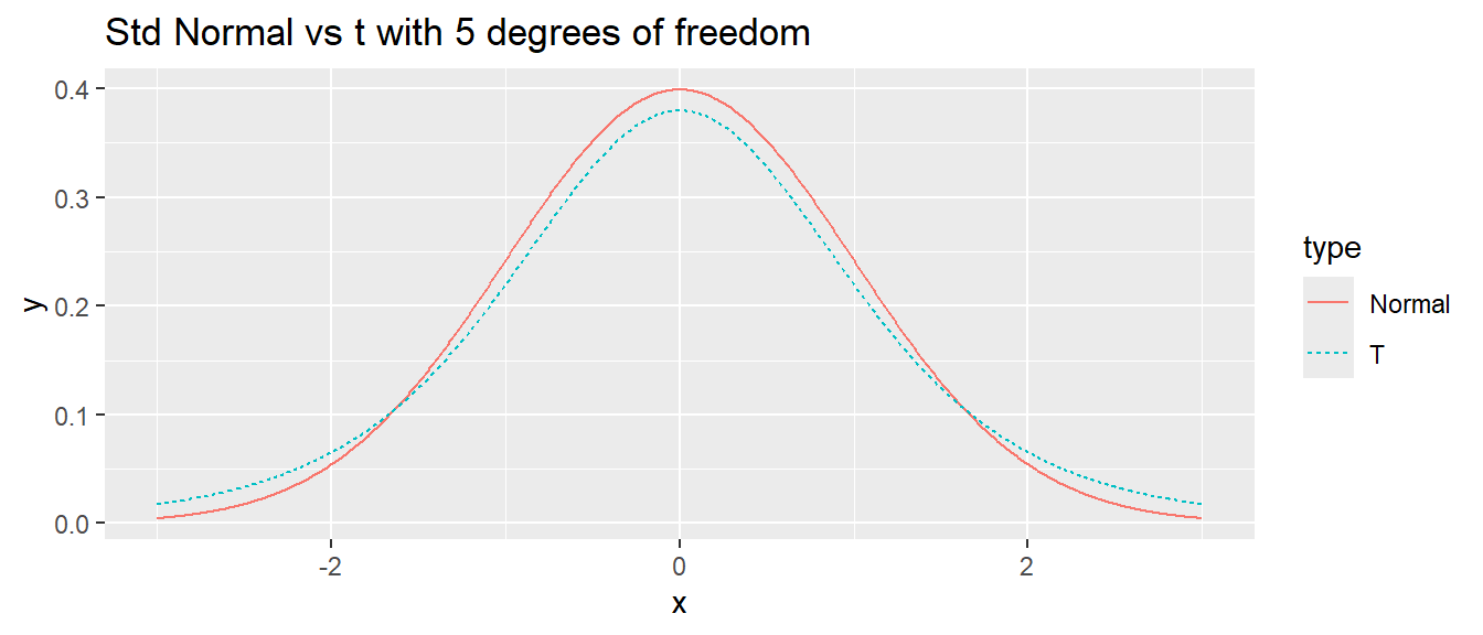
a) Use a for loop to create similar graphs for degrees of freedom \(2,3,4,\dots,29,30\).
b) In retrospect, perhaps we didn’t need to produce all of those. Rewrite your loop so that we only produce graphs for \(\left\{ 2,3,4,5,10,15,20,25,30\right\}\) degrees of freedom. Hint: you can just modify the vector in the for statement to include the desired degrees of freedom.
Exercise 4
It is very common to run simulation studies to estimate probabilities that are difficult to work out. The game is to roll a pair of 6-sided dice 24 times. If a “double-sixes” comes up on any of the 24 rolls, the player wins. What is the probability of winning?
a) We can simulate rolling two 6-sided dice using the sample() function with the replace=TRUE option. Read the help file on sample() to see how to sample from the numbers \(1,2,\dots,6\). Sum those two die rolls and save it as throw.
b) Write a for{} loop that wraps your code from part (a) and then tests if any of the throws of dice summed to 12. Read the help files for the functions any() and all(). Your code should look something like the following:
throws <- NULL
for( i in 1:24 ){
  throws[i] <- ??????  # Your part (a) code goes here
}
game <- any( throws == 12 ) # Gives a TRUE/FALSE value
c) Wrap all of your code from part (b) in another for(){} loop that you run 10,000 times. Save the result of each game in a games vector that will have 10,000 elements that are either TRUE/FALSE depending on the outcome of that game. You’ll need to initialize the games vector to NULL and modify your part (b) code to save the result into some location in the vector games.
d) Finally, calculate win percentage by taking the average of the games vector.